- What is going on?
- Where to get the code and data?
- Import data with readxl
- OK, first let’s remove the notes.
- However, we aren’t done. The data is “wide” instead of “long” and we have mixed session IDs (Amp 1-3 and Angle 1-3) with the value type.
- Now we need to extract the session (1,2,3) and the test type (Amp or Angle)
- Now we have two value types (Angle and Amplitude) in one column. So we need to go from long to wide to split them apart.
- Putting it all together and saving so we don’t have to see this big code block later.
- First plot. Does this work?
- But wait, this is a polar plot….
- Not bad, but we have a lot of little things to do.
- Yeah, so we need to tell ggplot what the range of values is.
- Cool, the range goes to 360 as expected. Still a few more things to do:
- Hmm, wrong way. (want 180 on the left) Let’s make it negative.
- OK, Final plot with some color and geom_point tweaking!
- sessionInfo
What is going on?
Where to get the code and data?
Rmarkdown document: https://github.com/davemcg/Let_us_plot/blob/master/001_polar_figure/polar_plot.Rmd Data: https://github.com/davemcg/Let_us_plot/blob/master/001_polar_figure/polar_values.xlsx
First time making a polar plot….let’s see if ggplot2 can do it.
Import data with readxl
library(tidyverse)## ── Attaching packages ────────────────────────────────────────────────────────────────────────────────── tidyverse 1.2.1 ──## ✔ ggplot2 3.0.0 ✔ purrr 0.2.5
## ✔ tibble 1.4.2 ✔ dplyr 0.7.6
## ✔ tidyr 0.8.1 ✔ stringr 1.3.1
## ✔ readr 1.1.1 ✔ forcats 0.3.0## ── Conflicts ───────────────────────────────────────────────────────────────────────────────────── tidyverse_conflicts() ──
## ✖ dplyr::filter() masks stats::filter()
## ✖ dplyr::lag() masks stats::lag()library(stringr)
polar_values <- readxl::read_xlsx('~/git/Let_us_plot/001_polar_figure/polar_values.xlsx')
polar_values## # A tibble: 8 x 8
## X__1 `Od Amp1` `Od Amp2` `Od Amp3` X__2 `Od Angle1` `Od Angle2`
## <chr> <dbl> <dbl> <dbl> <lgl> <dbl> <dbl>
## 1 3 2.1 3.01 2.96 NA 66 67.7
## 2 5 1.56 1.36 1.54 NA 19.6 14.7
## 3 14 4.79 4.73 4.72 NA 360. 353.
## 4 15 0.35 0.32 0.3 NA 257. 234.
## 5 18 0.91 0.83 1.12 NA 350. 344.
## 6 <NA> NA NA NA NA NA NA
## 7 1,2,3 are t… NA NA NA NA NA NA
## 8 Amp and Ang… NA NA NA NA NA NA
## # ... with 1 more variable: `Od Angle3` <dbl>OK, first let’s remove the notes.
We first slice the first 5 rows, then fix the encoding for Od Amp1, then remove the empty column in between
polar_values <- polar_values %>%
  slice(1:5) %>%
  mutate(Patient=as.factor(X__1)) %>%
  select(Patient,`Od Amp1`:`Od Amp3`, `Od Angle1`:`Od Angle3`)
polar_values
## # A tibble: 5 x 7
## Patient `Od Amp1` `Od Amp2` `Od Amp3` `Od Angle1` `Od Angle2`
## <fct> <dbl> <dbl> <dbl> <dbl> <dbl>
## 1 3 2.1 3.01 2.96 66 67.7
## 2 5 1.56 1.36 1.54 19.6 14.7
## 3 14 4.79 4.73 4.72 360. 353.
## 4 15 0.35 0.32 0.3 257. 234.
## 5 18 0.91 0.83 1.12 350. 344.
## # ... with 1 more variable: `Od Angle3` <dbl>However, we aren’t done. The data is “wide” instead of “long” and we have mixed session IDs (Amp 1-3 and Angle 1-3) with the value type.
Let’s first deal with the wide issue. If we google “R wide to long” we find this page near the top http://www.cookbook-r.com/Manipulating_data/Converting_data_between_wide_and_long_format/ which tells us that gather is the function we want.
Test_Session is the name for the column containing Od Amp1 to Od Angle Value is the name for the column holding the test measurements.
polar_values %>%
  gather(Test_Session, Value, `Od Amp1`:`Od Angle3`)
## # A tibble: 30 x 3
## Patient Test_Session Value
## <fct> <chr> <dbl>
## 1 3 Od Amp1 2.1
## 2 5 Od Amp1 1.56
## 3 14 Od Amp1 4.79
## 4 15 Od Amp1 0.35
## 5 18 Od Amp1 0.91
## 6 3 Od Amp2 3.01
## 7 5 Od Amp2 1.36
## 8 14 Od Amp2 4.73
## 9 15 Od Amp2 0.32
## 10 18 Od Amp2 0.83
## # ... with 20 more rowsNow we need to extract the session (1,2,3) and the test type (Amp or Angle)
We will use the fact that the session is always at the end to our advantage.
The str_sub function from the stringr package allows you to pick ‘negative’ positions in the string. So we pick last value and the first to the second last position to get what we need.
polar_values %>%
  gather(Test_Session, Value, `Od Amp1`:`Od Angle3`) %>%
  mutate(Session = str_sub(Test_Session, -1), Test = str_sub(Test_Session,1,-2))
## # A tibble: 30 x 5
## Patient Test_Session Value Session Test
## <fct> <chr> <dbl> <chr> <chr>
## 1 3 Od Amp1 2.1 1 Od Amp
## 2 5 Od Amp1 1.56 1 Od Amp
## 3 14 Od Amp1 4.79 1 Od Amp
## 4 15 Od Amp1 0.35 1 Od Amp
## 5 18 Od Amp1 0.91 1 Od Amp
## 6 3 Od Amp2 3.01 2 Od Amp
## 7 5 Od Amp2 1.36 2 Od Amp
## 8 14 Od Amp2 4.73 2 Od Amp
## 9 15 Od Amp2 0.32 2 Od Amp
## 10 18 Od Amp2 0.83 2 Od Amp
## # ... with 20 more rowsNow we have two value types (Angle and Amplitude) in one column. So we need to go from long to wide to split them apart.
We drop the now useless Test_Session column, grab the session number from the end with str_sub, then us the spread function to use the Test and Value columns to get it wide.
polar_values %>%
  gather(Test_Session, Value, `Od Amp1`:`Od Angle3`) %>%
  mutate(Session = str_sub(Test_Session, -1), Test = str_sub(Test_Session,1,-2)) %>%
  select(-Test_Session) %>%
  spread(Test, Value)
## # A tibble: 15 x 4
## Patient Session `Od Amp` `Od Angle`
## <fct> <chr> <dbl> <dbl>
## 1 14 1 4.79 360.
## 2 14 2 4.73 353.
## 3 14 3 4.72 353.
## 4 15 1 0.35 257.
## 5 15 2 0.32 234.
## 6 15 3 0.3 276.
## 7 18 1 0.91 350.
## 8 18 2 0.83 344.
## 9 18 3 1.12 349.
## 10 3 1 2.1 66
## 11 3 2 3.01 67.7
## 12 3 3 2.96 65.7
## 13 5 1 1.56 19.6
## 14 5 2 1.36 14.7
## 15 5 3 1.54 360.Boom. Mic drop.
Putting it all together and saving so we don’t have to see this big code block later.
reformatted_values <-
  polar_values %>%
  gather(Test_Session, Value, `Od Amp1`:`Od Angle3`) %>%
  mutate(Session = str_sub(Test_Session, -1), Test = str_sub(Test_Session,1,-2)) %>%
  select(-Test_Session) %>%
  spread(Test, Value)

reformatted_values
## # A tibble: 15 x 4
## Patient Session `Od Amp` `Od Angle`
## <fct> <chr> <dbl> <dbl>
## 1 14 1 4.79 360.
## 2 14 2 4.73 353.
## 3 14 3 4.72 353.
## 4 15 1 0.35 257.
## 5 15 2 0.32 234.
## 6 15 3 0.3 276.
## 7 18 1 0.91 350.
## 8 18 2 0.83 344.
## 9 18 3 1.12 349.
## 10 3 1 2.1 66
## 11 3 2 3.01 67.7
## 12 3 3 2.96 65.7
## 13 5 1 1.56 19.6
## 14 5 2 1.36 14.7
## 15 5 3 1.54 360.First plot. Does this work?
reformatted_values %>% ggplot(aes(y=`Od Amp`, x=`Od Angle`)) + geom_point()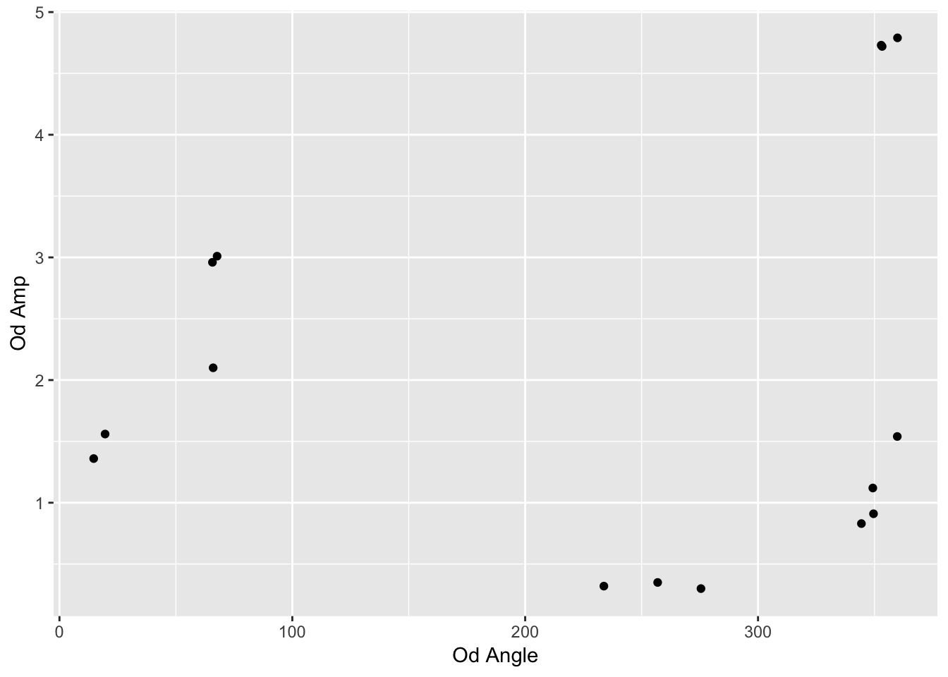
But wait, this is a polar plot….
Fortunately ggplot has a function to transform cartesian values into polar values: coord_polar
reformatted_values %>% ggplot(aes(y=`Od Amp`, x=`Od Angle`)) + coord_polar() + geom_point()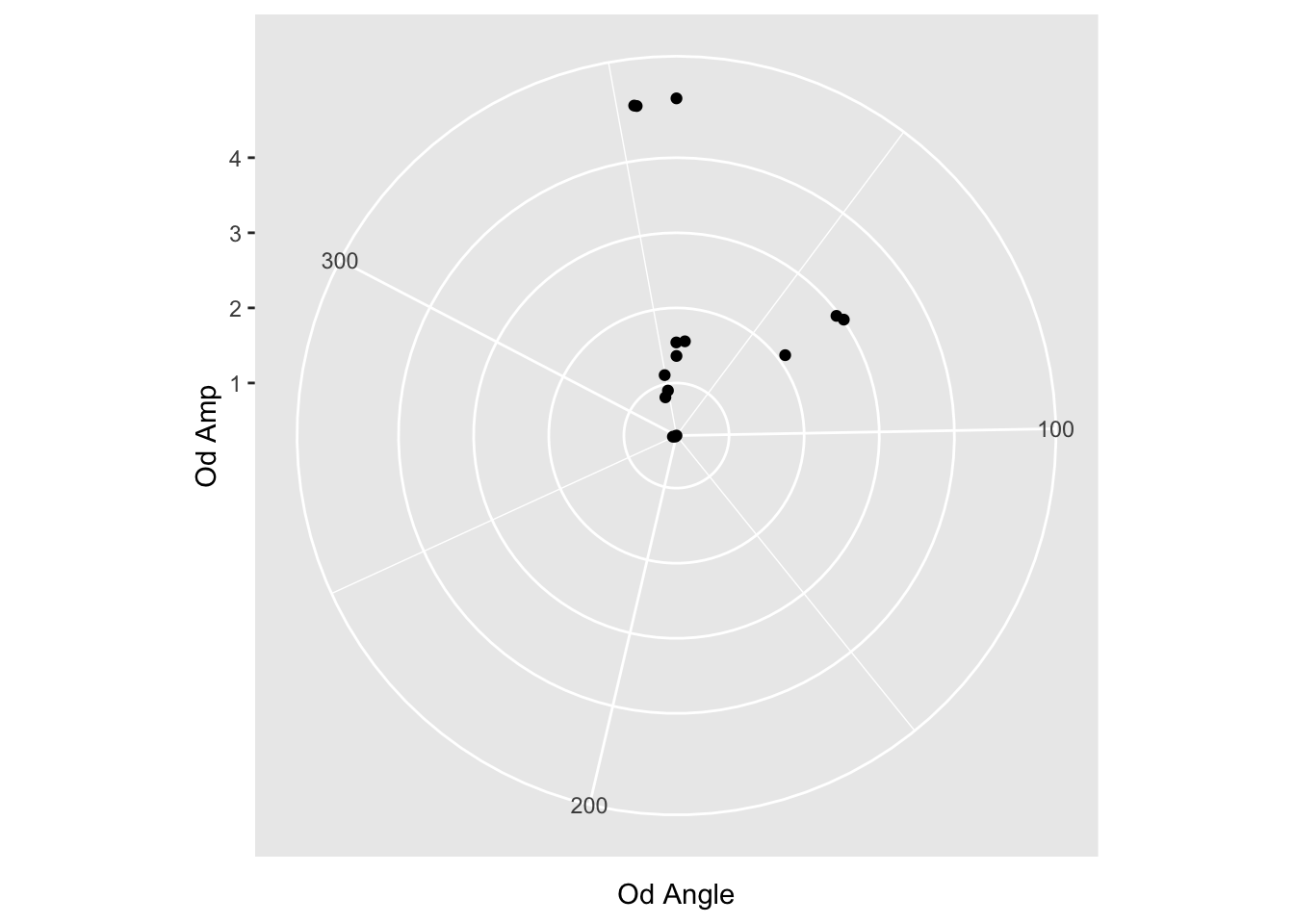
Not bad, but we have a lot of little things to do.
First, I’m suspicious that the ranges of values is from the smallest to the largest. Or maybe 0 to the largest. We can test this by filtering out the bigger values.
reformatted_values %>%
  filter(`Od Angle` < 300) %>%
  ggplot(aes(y=`Od Amp`, x=`Od Angle`)) + coord_polar() + geom_point()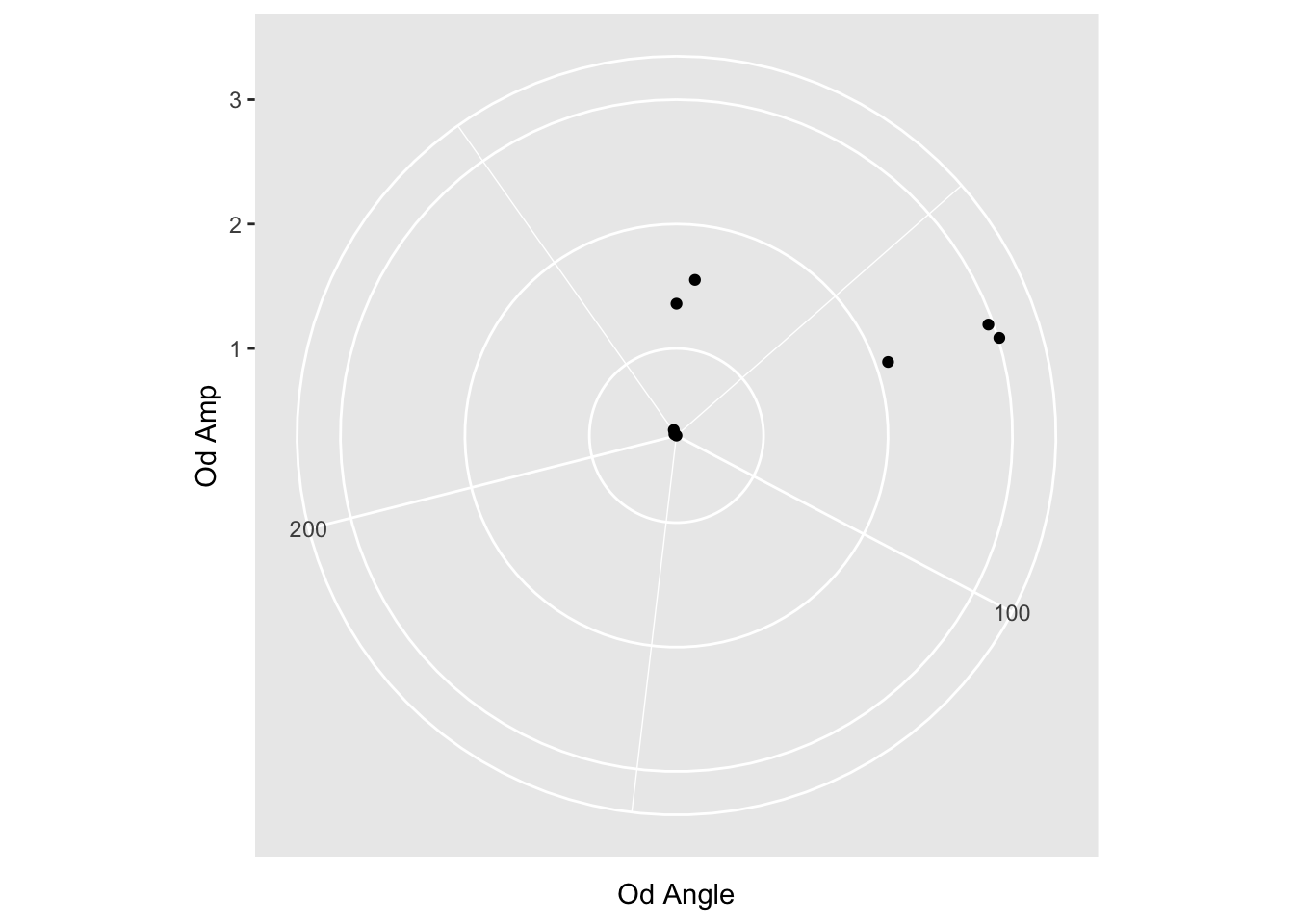
Yeah, so we need to tell ggplot what the range of values is.
reformatted_values %>% filter(`Od Angle` < 300) %>%
  ggplot(aes(y=`Od Amp`, x=`Od Angle`)) +
  coord_polar() +
  geom_point() +
scale_x_continuous(limits=c(0,360), breaks = c(0,30,60,90,120,150,180,210,240,270,300,330)) 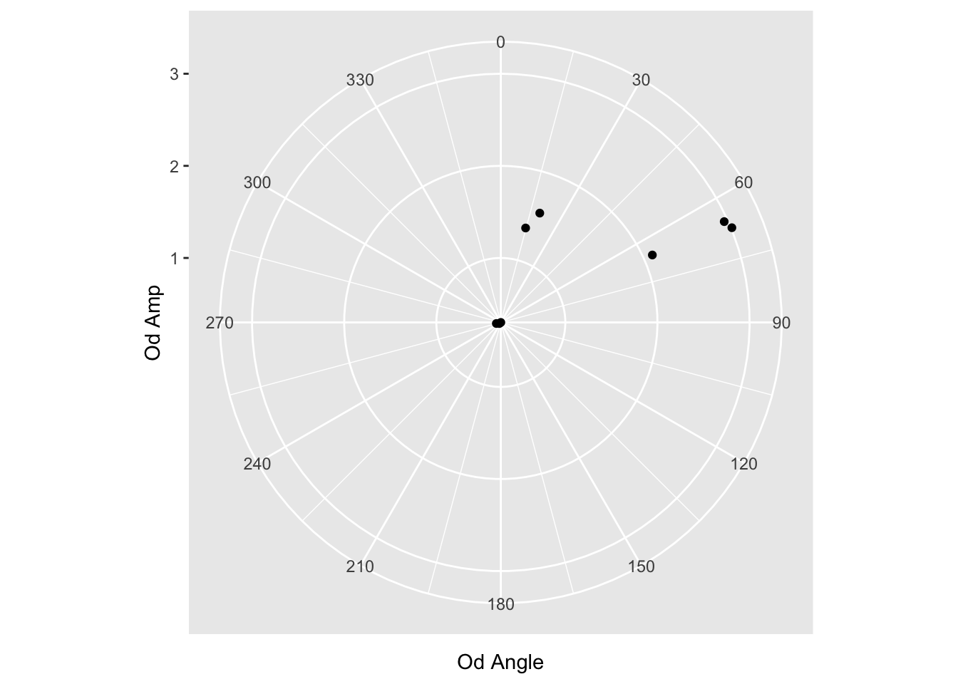
Cool, the range goes to 360 as expected. Still a few more things to do:
- Rotate the start point so 90 is the top
- Change directions of values from CW to CCW
- Add color and prettify
We examine the coord_polar options (type ?coord_polar in the R console) and see that start and direction are options. We want to shift 90 degrees…but the start parameter is in radians. Some quick googling let’s us know that 90 degree ~ 1.57 radians. Let’s use that. And -1 for direction to make it counter clockwise.
reformatted_values %>%
  ggplot(aes(y=`Od Amp`, x=`Od Angle`)) +
  coord_polar(start = 1.57, direction = -1) +
  geom_point() +
scale_x_continuous(limits=c(0,360), breaks = c(0,30,60,90,120,150,180,210,240,270,300,330)) 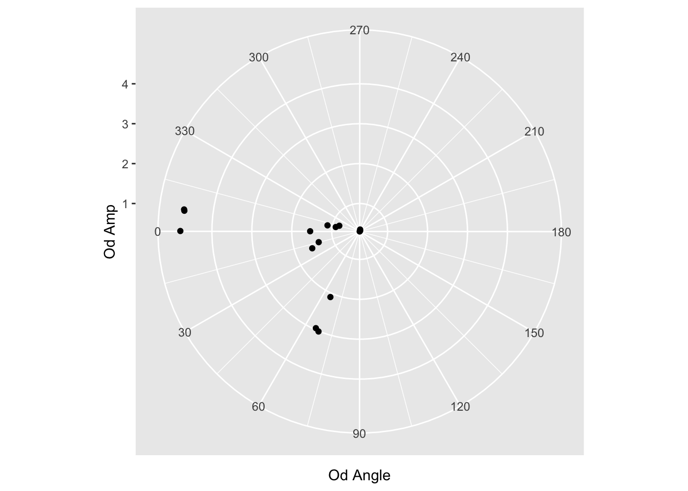
Hmm, wrong way. (want 180 on the left) Let’s make it negative.
reformatted_values %>%
  ggplot(aes(y=`Od Amp`, x=`Od Angle`)) +
  coord_polar(start = -1.57, direction = -1) +
  geom_point() +
scale_x_continuous(limits=c(0,360), breaks = c(0,30,60,90,120,150,180,210,240,270,300,330)) 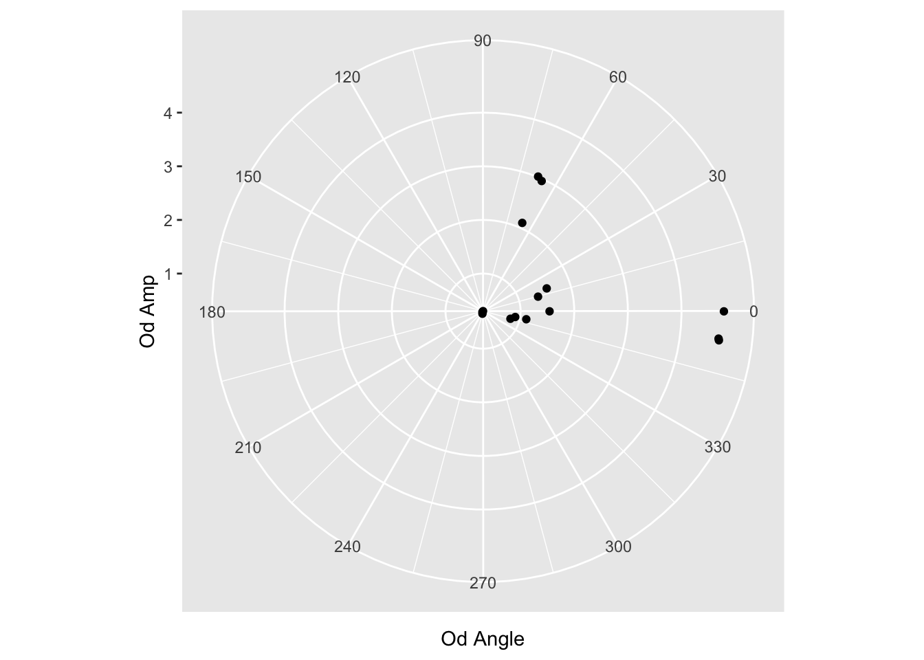
OK, Final plot with some color and geom_point tweaking!
theme_bw makes the background white instead of gray, which I prefer
alpha in geom_point makes the points semi-transparent
scale_colour_brewer is a nicer color palette, in my opinion
colour and shape in ggplot() gives us color and shape for the patients and three sessions
reformatted_values %>% ggplot(aes(y=`Od Amp`, x=`Od Angle`, colour=Patient, shape=Session)) +
  coord_polar(start = -1.57, direction = -1) +
  geom_point(size=3, alpha=0.7) +
  theme_bw() +
  scale_x_continuous(limits=c(0,360), breaks = c(0,30,60,90,120,150,180,210,240,270,300,330)) +
  scale_color_brewer(palette ='Set1') + xlab('Angle') + ylab('Amplitude') + ggtitle('OD')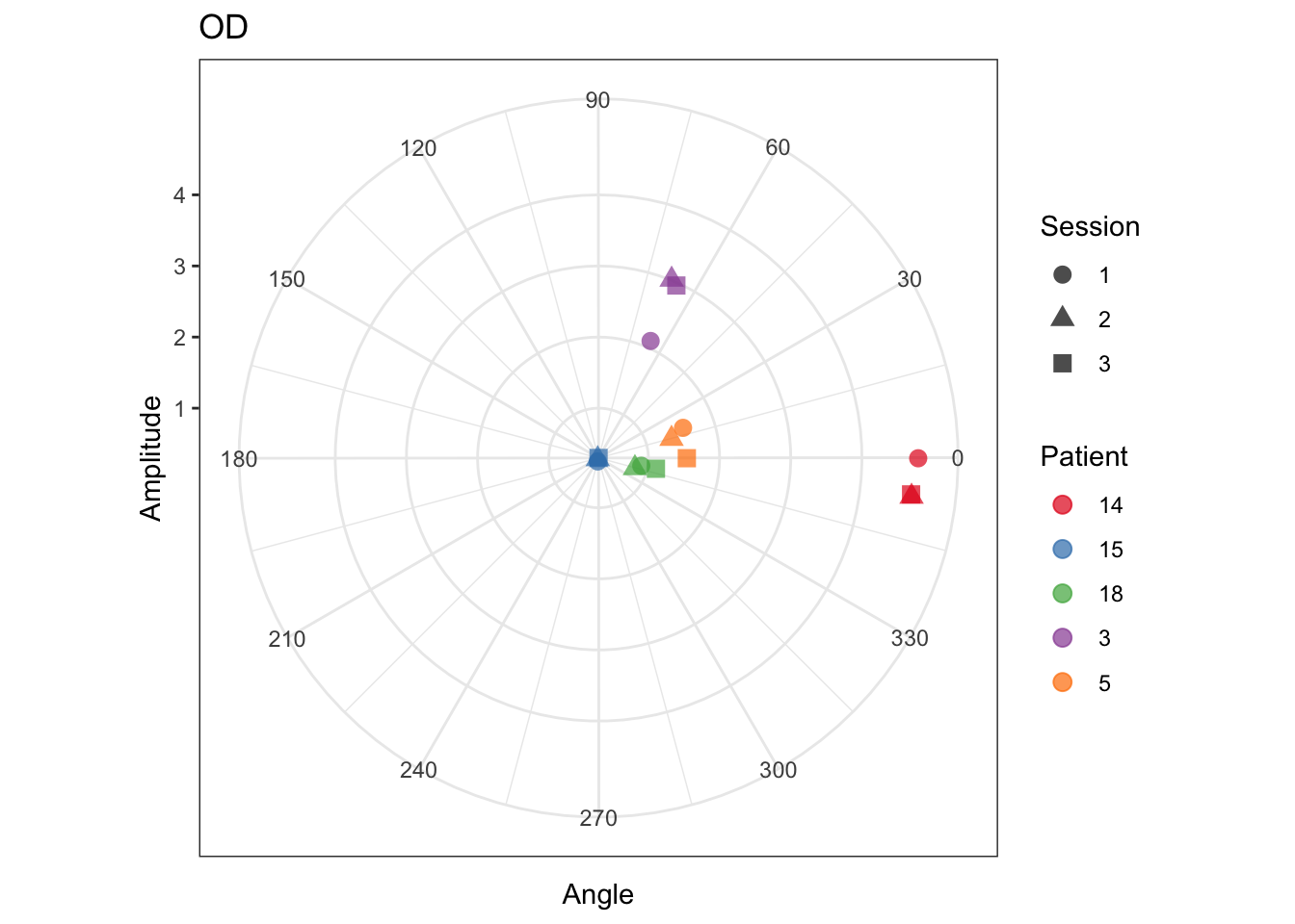
sessionInfo
sessionInfo()## R version 3.5.0 (2018-04-23)
## Platform: x86_64-apple-darwin15.6.0 (64-bit)
## Running under: macOS High Sierra 10.13.6
##
## Matrix products: default
## BLAS: /Library/Frameworks/R.framework/Versions/3.5/Resources/lib/libRblas.0.dylib
## LAPACK: /Library/Frameworks/R.framework/Versions/3.5/Resources/lib/libRlapack.dylib
##
## locale:
## [1] en_US.UTF-8/en_US.UTF-8/en_US.UTF-8/C/en_US.UTF-8/en_US.UTF-8
##
## attached base packages:
## [1] stats graphics grDevices utils datasets methods base
##
## other attached packages:
## [1] bindrcpp_0.2.2 forcats_0.3.0 stringr_1.3.1 dplyr_0.7.6
## [5] purrr_0.2.5 readr_1.1.1 tidyr_0.8.1 tibble_1.4.2
## [9] ggplot2_3.0.0 tidyverse_1.2.1
##
## loaded via a namespace (and not attached):
## [1] tidyselect_0.2.4 xfun_0.3 reshape2_1.4.3
## [4] haven_1.1.1 lattice_0.20-35 colorspace_1.3-2
## [7] htmltools_0.3.6 yaml_2.1.19 utf8_1.1.4
## [10] rlang_0.2.1 pillar_1.2.3 withr_2.1.2
## [13] foreign_0.8-70 glue_1.2.0 RColorBrewer_1.1-2
## [16] modelr_0.1.2 readxl_1.1.0 bindr_0.1.1
## [19] plyr_1.8.4 munsell_0.4.3 blogdown_0.8
## [22] gtable_0.2.0 cellranger_1.1.0 rvest_0.3.2
## [25] psych_1.8.4 evaluate_0.10.1 labeling_0.3
## [28] knitr_1.20 parallel_3.5.0 broom_0.4.4
## [31] Rcpp_0.12.17 backports_1.1.2 scales_0.5.0
## [34] jsonlite_1.5 mnormt_1.5-5 hms_0.4.2
## [37] digest_0.6.15 stringi_1.2.2 bookdown_0.7
## [40] grid_3.5.0 rprojroot_1.3-2 cli_1.0.0
## [43] tools_3.5.0 magrittr_1.5 lazyeval_0.2.1
## [46] crayon_1.3.4 pkgconfig_2.0.1 xml2_1.2.0
## [49] lubridate_1.7.4 assertthat_0.2.0 rmarkdown_1.10
## [52] httr_1.3.1 rstudioapi_0.7 R6_2.2.2
## [55] nlme_3.1-137 compiler_3.5.0