Introduction
This is a barebones (but detailed enough, I hope) discussion of how to take a bam file, extract base pair resolution coverage data, then finagle the data into coverage plots by gene and exon. No data will be given for the below code. I’m not sharing a bam file. Also, not much point to sharing the bed, HGNC name, and gtf file, as there’s a decent chance they won’t work for your bam.
Call mosdepth on bam to calculate bp-specific read depth
mosdepth, by default, will generate base pair resolution coverage across the entire genome. Another fantastic tool from Brent Peterson and Aaron Quinlan (some point I’ll do a gushy post on all of the useful tools Quinlan and company have made).
mosdepth will run very quickly (minutes instead of hours), compared to bedtools genomecov.
# bash
sinteractive --cpus-per-task 16
module load mosdepth
mosdepth -t 16 41001412010527 41001412010527_realigned_recal.bam &
Intersect base pair depth info with transcript and exon number
The intersect is to select regions overlapping exons and to label them with the transcript name and exon number present in gencode_genes_v27lift37.codingExons.ensembl.bed.gz. See the code below for how to make your own.
# bash

# gencode_genes_v27lift37.codingExons.bed was downloaded from the UCSC table browser from genocde gene v27lift37 and 'coding exons' with 0 padding were selected as the output for the bed file
# my https://github.com/davemcg/ChromosomeMappings/ convert_notation.py script was then used to convert the UCSC notation in ensembl notation, which my bam uses
# files in biowulf2:/data/mcgaugheyd/genomes/GRCh37/
module load bedtools
~/git/ChromosomeMappings/convert_notation.py -c ~/git/ChromosomeMappings/GRCh37_gencode2ensembl.txt -f gencode_genes_v27lift37.codingExons.bed | sort -k1,1 -k2,2n | gzip > gencode_genes_v27lift37.codingExons.ensembl.bed.gz
bedtools intersect -wa -wb -a 41001412010527.per-base.bed.gz -b /data/mcgaugheyd/genomes/GRCh37/gencode_genes_v27lift37.codingExons.ensembl.bed.gz | bgzip  > 41001412010527.per-base.labeled.bed.gz &
Now it’s R time!
Prepare Metadata
You’ll need HGNC <-> Ensembl Transcript converter and the Gencode GTF
The first file is used to match gene ‘names’ with ensembl transcript ID
The second file is used to semi-accurately pick the ‘canonical’ transcript for a gene (pick the appris transcript, then the longest)
library(data.table)
library(tidyverse)
## ── Attaching packages ────────────────────────────────────────────────────────────────────────────────────────────────────────────────────────────────────────────── tidyverse 1.2.1 ──## ✔ ggplot2 3.0.0 ✔ purrr 0.2.4
## ✔ tibble 1.4.2 ✔ dplyr 0.7.6
## ✔ tidyr 0.8.1 ✔ stringr 1.3.1
## ✔ readr 1.1.1 ✔ forcats 0.3.0## ── Conflicts ───────────────────────────────────────────────────────────────────────────────────────────────────────────────────────────────────────────────── tidyverse_conflicts() ──
## ✖ dplyr::between() masks data.table::between()
## ✖ dplyr::filter() masks stats::filter()
## ✖ dplyr::first() masks data.table::first()
## ✖ dplyr::lag() masks stats::lag()
## ✖ dplyr::last() masks data.table::last()
## ✖ purrr::transpose() masks data.table::transpose()library(cowplot)##
## Attaching package: 'cowplot'## The following object is masked from 'package:ggplot2':
##
## ggsavelibrary(stringr)
metadata <- fread('gzcat ~/GenomicData/gencode.v27lift37.metadata.HGNC.gz', header=F)
colnames(metadata) <- c('Transcript','Name')
gencode <- fread('gzcat ~/GenomicData/gencode.v27lift37.basic.annotation.gtf.gz', header=F, skip=4)
gencode2 <- gencode %>% filter(V3=='transcript') %>%
filter(grepl('appris_principal', V9)) %>%
rowwise() %>%
mutate(Transcript = str_extract(V9,'ENST\\d{11}\\.\\d+'), # use regex to graph ensembl transcript
Gene = str_extract(V9, 'gene_name\\s\\".*?;'), # and the gene name
Size=V5-V4) %>%
separate(Gene, c('skip','Name','skip2'),'\"') %>% # now you have to remove the 'gene name' part
select(-skip, -skip2) %>%
group_by(Name) %>% top_n(1)## Selecting by SizeLoad mosdepth / bedtools intersect data and prep
Label coverage chunks with the depth of their coverage with case_when and extract the transcript name and exon number with a bunch of separate commands
depth_data <- fread('gzcat ~/Desktop/41001412010527.per-base.labeled.bed.gz')
dd_processed <- depth_data %>%
  separate(V8, c('Transcript','Rest'), '_cds_') %>%
  separate(Rest, c('Before','Stuff'),'_chr') %>%
  separate(Before, c('Exon Number','Num2'),sep='_') %>%
  mutate(Depth = case_when(V4 < 10 ~ '< 10 Reads',
                           V4 < 20 ~ '< 20 Reads',
                           TRUE ~ '>= 20 Reads')) %>%
  mutate(Depth=factor(Depth, levels=c('< 10 Reads','< 20 Reads','>= 20 Reads'))) %>%
  mutate(Transcript=case_when(grepl('_',Transcript) ~ gsub('_.','',Transcript),
                              TRUE ~ Transcript)) %>%
  select(Chr=V1, Start=V2, End=V3, Read_Depth=V4, Transcript, Strand=V10, Depth, `Exon Number`, ExonStart=V6, ExonEnd=V7)

dd_processed <- left_join(dd_processed, metadata, by=c('Transcript'))
Plot Maker, version 1
Faceted by exon. One plot per gene and using cowplot to glue them together
genes <- c('PAX6','ABCA4','NRL','CRX','RPGR')
transcripts = gencode2 %>% filter(Name %in% genes) %>% pull(Transcript)

# set a custom color that will work even if a category is missing
scale_colour_custom <- function(...){
  ggplot2:::manual_scale('colour',
                         values = setNames(c('darkred', 'red', 'black'),
                                           c('< 10 Reads','< 20 Reads','>= 20 Reads')),
                         ...)
}

plot_maker <- function(tx){
  num_of_exons <- dd_processed %>% filter(Transcript==tx) %>% pull(`Exon Number`) %>% as.numeric() %>% max()
  gene_name <-  dd_processed %>% filter(Transcript==tx) %>% pull(Name) %>% unique()
  # expand to create a row for each sequence and fill in previous values
  dd_processed %>% filter(Transcript==tx) %>% group_by(`Exon Number`) %>%
    expand(Start=full_seq(c(Start,End),1)) %>%
    left_join(.,  dd_processed %>% filter(Transcript==tx)) %>% # create one row per base position, grouped by Exon Number https://stackoverflow.com/questions/42866119/fill-missing-values-in-data-frame-using-dplyr-complete-within-groups
    fill(Chr:Name) %>% # fill missing values https://stackoverflow.com/questions/40040834/r-replace-na-with-previous-or-next-value-by-group-using-dplyr
    ungroup() %>% # drop the exon number grouping, so I can mutate below
    mutate(`Exon Number`= factor(`Exon Number`,levels=0:num_of_exons)) %>% # Ah, reordering. I need it to be a factor, but then I have to explicitly give the order
    mutate(Depth = factor(Depth, levels=c('< 10 Reads','< 20 Reads','>= 20 Reads'))) %>%  # create three categories for coloring
    ggplot(aes(x=Start, xend=End, y=Read_Depth, yend=Read_Depth, colour=Depth)) +
    facet_wrap(~`Exon Number`, scales = 'free_x', nrow=1, strip.position = 'bottom') +
    geom_point(size=0.1) + theme_minimal()+ scale_colour_custom() +  # use my custom color set above for my three categories
    theme(axis.text.x=element_blank(),
          axis.ticks.x = element_blank(),
          panel.grid.minor = element_blank(),
          panel.grid.major.x = element_blank(),
          legend.position = 'none') +
    ylab('Depth') +
    xlab(paste0(gene_name[1]))
}

# little for loop to roll through the transcripts and make plot, storing in a list
plots <- list()
for (i in transcripts){
  plots[[i]] <- plot_maker(i)
}
## Joining, by = c("Exon Number", "Start")
## Joining, by = c("Exon Number", "Start")
## Joining, by = c("Exon Number", "Start")
## Joining, by = c("Exon Number", "Start")
## Joining, by = c("Exon Number", "Start")legend <- get_legend(plots[[names(plots)[1]]] + theme(legend.position='right'))
# cowplot can take a list and glue the plots together
# I'm commenting out the below line because blogdown makes it too damn small. You need to run it to make the plot
# plot_grid(plot_grid(plotlist = plots, ncol=1, hjust=-2), legend, ncol=2, rel_widths = c(5,0.5))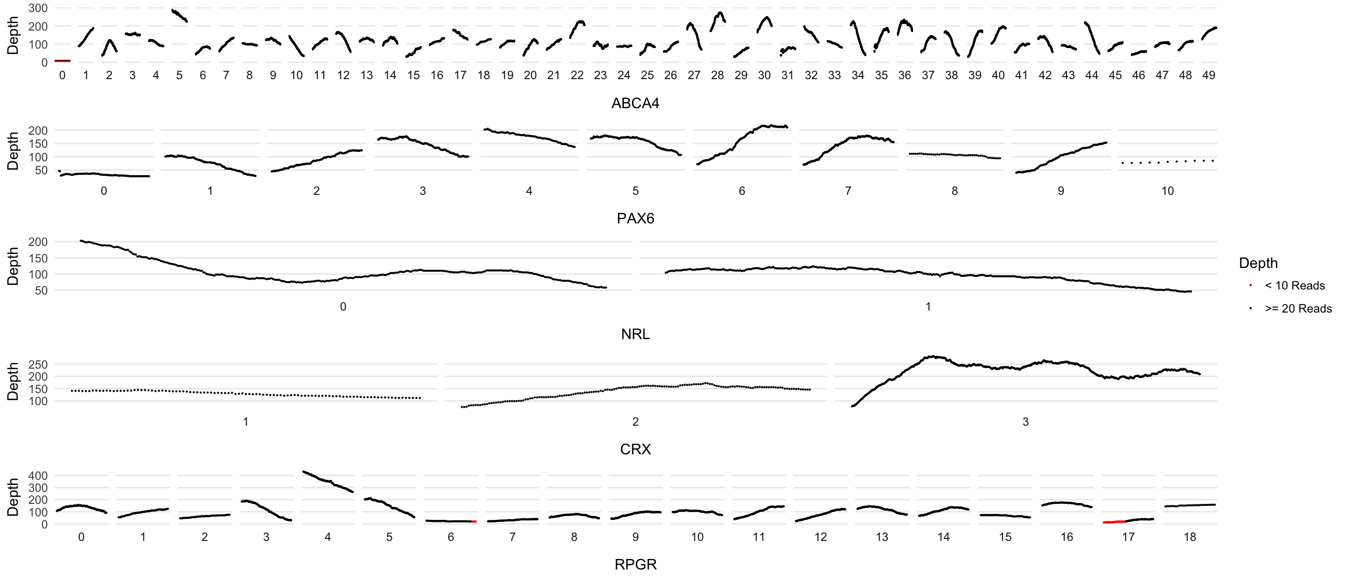
Version 2
A bit tighter. Recalculates coordinates to glue all of the exons together in one plot. I can facet by gene. A bit harder to read, but is more accurate as the exons and gene lengths are proportional
genes <- c('PAX6','ABCA4','NRL','CRX','RPGR')
tx = gencode2 %>% filter(Name %in% genes) %>% pull(Transcript)

dd_expanded <- dd_processed %>% filter(Transcript %in% tx) %>% group_by(Transcript, `Exon Number`) %>%
  expand(Start=full_seq(c(Start,End),1)) %>%
  left_join(.,  dd_processed %>% filter(Transcript %in% tx)) %>% # create one row per base position, grouped by Exon Number https://stackoverflow.com/questions/42866119/fill-missing-values-in-data-frame-using-dplyr-complete-within-groups
  fill(Chr:Name) # fill missing values https://stackoverflow.com/questions/40040834/r-replace-na-with-previous-or-next-value-by-group-using-dplyr
## Joining, by = c("Transcript", "Exon Number", "Start")dd_expanded <- dd_expanded %>% group_by(Name) %>% mutate(Pos = 1:n())
even_odds_marking <- dd_expanded %>% group_by(Name, `Exon Number`) %>% summarise(Start=min(Pos), End=max(Pos)) %>% mutate(Exon = case_when(as.numeric(`Exon Number`) %% 2 == 0 ~ 'even', TRUE ~ 'odd'))
plot_data<-bind_rows(dd_expanded,even_odds_marking)
ggplot() +
geom_point(data = plot_data %>% filter(is.na(Exon)), aes(x=Pos, y=Read_Depth, colour=Depth),size=0.1) +
facet_wrap(~Name, ncol=1) +
geom_rect(data = plot_data %>% filter(!is.na(Exon)), aes(xmin=Start, xmax=End, ymin=-Inf, ymax=Inf, fill=Exon)) +
scale_fill_manual(values = alpha(c("gray", "white"), .3)) +
scale_colour_custom() +
theme_minimal() +
theme(axis.text.x=element_blank(),
axis.ticks.x = element_blank(),
panel.grid.minor = element_blank(),
panel.grid.major.x = element_blank())+
guides(fill=FALSE) +
ylab('Read Depth') 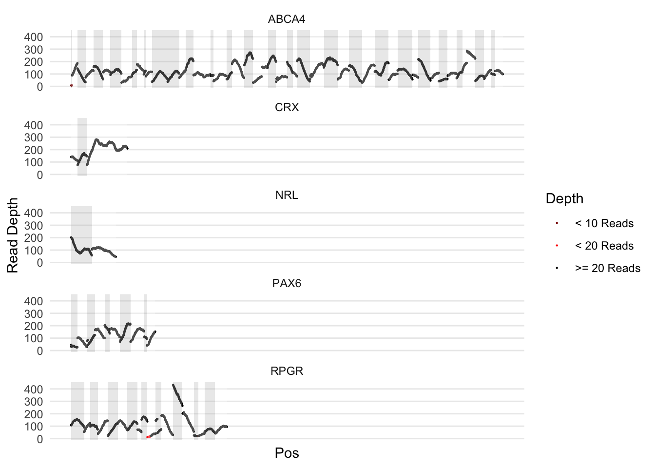
sessionInfo()
devtools::session_info()## Session info -------------------------------------------------------------## setting value
## version R version 3.5.0 (2018-04-23)
## system x86_64, darwin15.6.0
## ui X11
## language (EN)
## collate en_US.UTF-8
## tz America/New_York
## date 2018-07-16## Packages -----------------------------------------------------------------## package * version date source
## assertthat 0.2.0 2017-04-11 CRAN (R 3.5.0)
## backports 1.1.2 2017-12-13 CRAN (R 3.5.0)
## base * 3.5.0 2018-04-24 local
## bindr 0.1.1 2018-03-13 CRAN (R 3.5.0)
## bindrcpp * 0.2.2 2018-03-29 CRAN (R 3.5.0)
## blogdown 0.8.1 2018-07-16 Github (rstudio/blogdown@d54c39a)
## bookdown 0.7 2018-02-18 CRAN (R 3.5.0)
## broom 0.4.4 2018-03-29 CRAN (R 3.5.0)
## cellranger 1.1.0 2016-07-27 CRAN (R 3.5.0)
## cli 1.0.0 2017-11-05 CRAN (R 3.5.0)
## colorspace 1.3-2 2016-12-14 CRAN (R 3.5.0)
## compiler 3.5.0 2018-04-24 local
## cowplot * 0.9.2 2017-12-17 CRAN (R 3.5.0)
## crayon 1.3.4 2017-09-16 CRAN (R 3.5.0)
## data.table * 1.11.4 2018-05-27 cran (@1.11.4)
## datasets * 3.5.0 2018-04-24 local
## devtools 1.13.5 2018-02-18 CRAN (R 3.5.0)
## digest 0.6.15 2018-01-28 CRAN (R 3.5.0)
## dplyr * 0.7.6 2018-06-29 cran (@0.7.6)
## evaluate 0.10.1 2017-06-24 CRAN (R 3.5.0)
## forcats * 0.3.0 2018-02-19 CRAN (R 3.5.0)
## foreign 0.8-70 2017-11-28 CRAN (R 3.5.0)
## ggplot2 * 3.0.0 2018-07-03 cran (@3.0.0)
## glue 1.2.0 2017-10-29 CRAN (R 3.5.0)
## graphics * 3.5.0 2018-04-24 local
## grDevices * 3.5.0 2018-04-24 local
## grid 3.5.0 2018-04-24 local
## gtable 0.2.0 2016-02-26 CRAN (R 3.5.0)
## haven 1.1.1 2018-01-18 CRAN (R 3.5.0)
## hms 0.4.2 2018-03-10 CRAN (R 3.5.0)
## htmltools 0.3.6 2017-04-28 CRAN (R 3.5.0)
## httr 1.3.1 2017-08-20 CRAN (R 3.5.0)
## jsonlite 1.5 2017-06-01 CRAN (R 3.5.0)
## knitr 1.20 2018-02-20 CRAN (R 3.5.0)
## labeling 0.3 2014-08-23 CRAN (R 3.5.0)
## lattice 0.20-35 2017-03-25 CRAN (R 3.5.0)
## lazyeval 0.2.1 2017-10-29 CRAN (R 3.5.0)
## lubridate 1.7.4 2018-04-11 CRAN (R 3.5.0)
## magrittr 1.5 2014-11-22 CRAN (R 3.5.0)
## memoise 1.1.0 2017-04-21 CRAN (R 3.5.0)
## methods * 3.5.0 2018-04-24 local
## mnormt 1.5-5 2016-10-15 CRAN (R 3.5.0)
## modelr 0.1.2 2018-05-11 CRAN (R 3.5.0)
## munsell 0.4.3 2016-02-13 CRAN (R 3.5.0)
## nlme 3.1-137 2018-04-07 CRAN (R 3.5.0)
## parallel 3.5.0 2018-04-24 local
## pillar 1.2.3 2018-05-25 CRAN (R 3.5.0)
## pkgconfig 2.0.1 2017-03-21 CRAN (R 3.5.0)
## plyr 1.8.4 2016-06-08 CRAN (R 3.5.0)
## psych 1.8.4 2018-05-06 CRAN (R 3.5.0)
## purrr * 0.2.4 2017-10-18 CRAN (R 3.5.0)
## R6 2.2.2 2017-06-17 CRAN (R 3.5.0)
## Rcpp 0.12.17 2018-05-18 CRAN (R 3.5.0)
## readr * 1.1.1 2017-05-16 CRAN (R 3.5.0)
## readxl 1.1.0 2018-04-20 CRAN (R 3.5.0)
## reshape2 1.4.3 2017-12-11 CRAN (R 3.5.0)
## rlang 0.2.1 2018-05-30 CRAN (R 3.5.0)
## rmarkdown 1.10 2018-06-11 cran (@1.10)
## rprojroot 1.3-2 2018-01-03 CRAN (R 3.5.0)
## rstudioapi 0.7 2017-09-07 CRAN (R 3.5.0)
## rvest 0.3.2 2016-06-17 CRAN (R 3.5.0)
## scales 0.5.0 2017-08-24 CRAN (R 3.5.0)
## stats * 3.5.0 2018-04-24 local
## stringi 1.2.2 2018-05-02 CRAN (R 3.5.0)
## stringr * 1.3.1 2018-05-10 CRAN (R 3.5.0)
## tibble * 1.4.2 2018-01-22 CRAN (R 3.5.0)
## tidyr * 0.8.1 2018-05-18 CRAN (R 3.5.0)
## tidyselect 0.2.4 2018-02-26 CRAN (R 3.5.0)
## tidyverse * 1.2.1 2017-11-14 CRAN (R 3.5.0)
## tools 3.5.0 2018-04-24 local
## utils * 3.5.0 2018-04-24 local
## withr 2.1.2 2018-03-15 CRAN (R 3.5.0)
## xfun 0.3 2018-07-06 cran (@0.3)
## xml2 1.2.0 2018-01-24 CRAN (R 3.5.0)
## yaml 2.1.19 2018-05-01 CRAN (R 3.5.0)