Introduction
The battle that we’ve all been waiting for. Excel vs. R. Bar plot versus a plot that actually shows the data.
Yeah, this isn’t a fair fight.
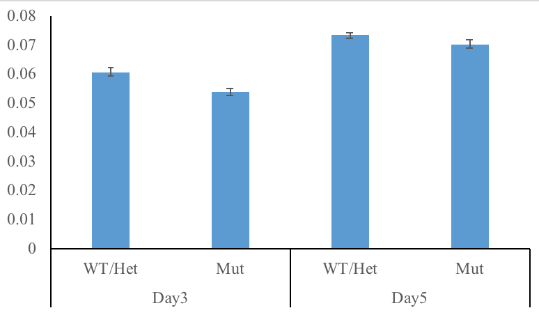
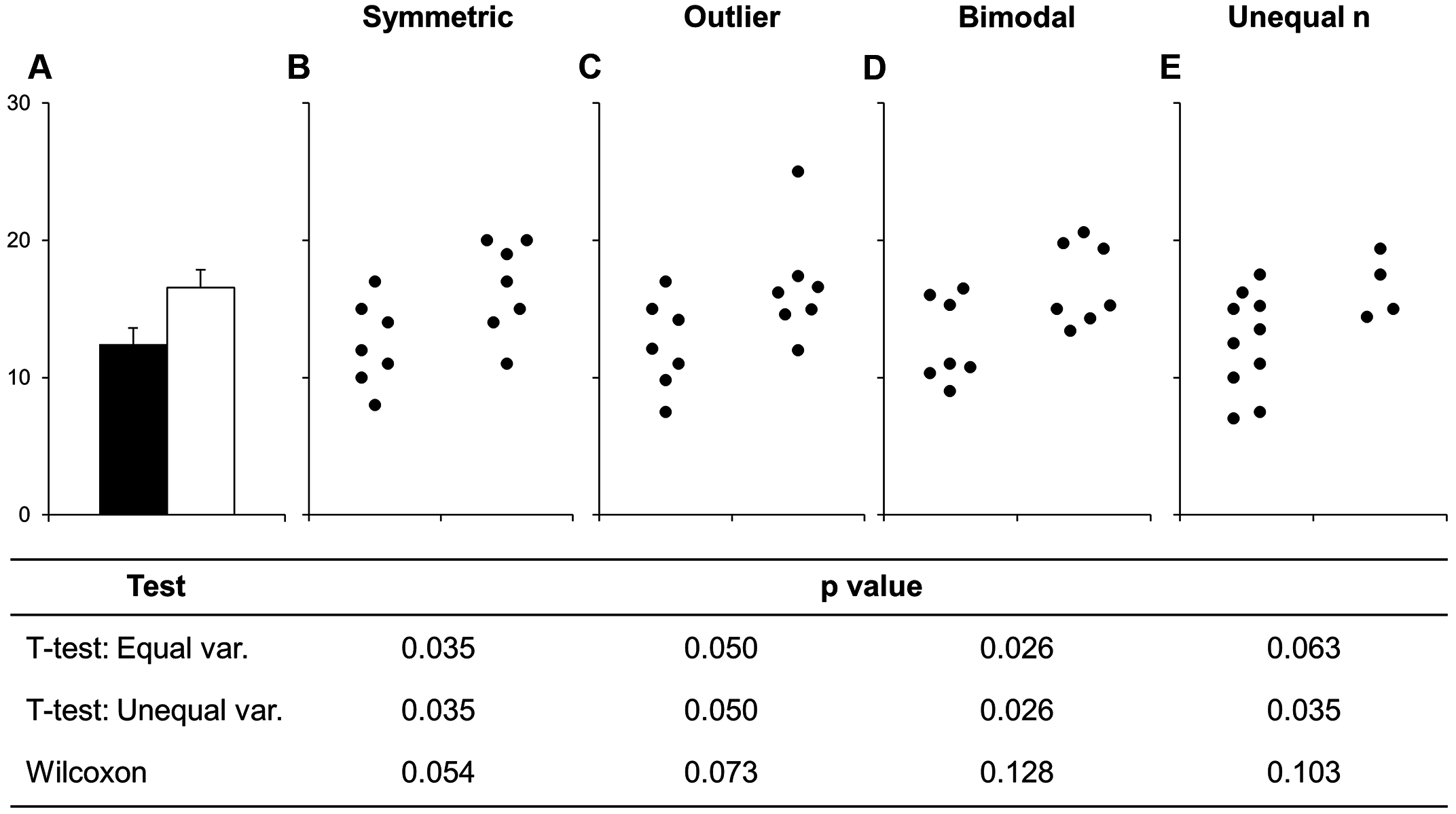
Bar plots are terrible. Why? Simple. They don’t show what your data looks like. A bar plot gives you zero idea how many data points there are. You can add error bars, but you don’t know if you are looking at standard error or standard deviation.
Box plots are much better. They display useful information like minimum, maximum, quartiles, and median. But they still can really mislead depending on how your data is structured.
Why do so many scientists keep using bar (or box) plots? Well, simple. Excel makes bar plots with one click. Excel can make box plots, but it is not easy.
Excel, as far as I can tell, can’t do what I’m about to show you: violin plots or box plots with the raw data displayed inline.
As a bonus, I made a short video to demonstrate how you can skip the below data cleaning in R with some clicking and dragging in Excel - then just plot in R.
Data
A variety of eye measurements between a wild-type zebrafish line and a mutant line.
You can get the excel file here
library(tidyverse)## ── Attaching packages ────────────────────────────────────────────────────────────────────────────────────────────────────────────────────────────────────────────── tidyverse 1.2.1 ──## ✔ ggplot2 3.0.0 ✔ purrr 0.2.4
## ✔ tibble 1.4.2 ✔ dplyr 0.7.6
## ✔ tidyr 0.8.1 ✔ stringr 1.3.1
## ✔ readr 1.1.1 ✔ forcats 0.3.0## Warning: package 'dplyr' was built under R version 3.5.1## ── Conflicts ───────────────────────────────────────────────────────────────────────────────────────────────────────────────────────────────────────────────── tidyverse_conflicts() ──
## ✖ dplyr::filter() masks stats::filter()
## ✖ dplyr::lag() masks stats::lag()library(ggsci)
library(ggbeeswarm)
micro <- readxl::read_xlsx('~/git/Let_us_plot/004_r_vs_excel/Compiled eye measurements.xlsx')
head(micro)## # A tibble: 6 x 13
## X__1 Day3 X__2 Day5 X__3 X__4 X__5 X__6 X__7 X__8 X__9 X__10
## <chr> <chr> <chr> <chr> <chr> <lgl> <lgl> <lgl> <chr> <chr> <chr> <chr>
## 1 Fish WT/Het Mut WT/H… Mut NA NA NA <NA> <NA> <NA> <NA>
## 2 1 6.099… 4.80… 7.29… 6.70… NA NA NA <NA> Day3 <NA> Day5
## 3 2 7.099… 5.29… 7.19… 8.20… NA NA NA <NA> WT/H… Mut WT/H…
## 4 3 0.05 5.39… 7.69… 7.09… NA NA NA avg 6.06… 5.37… 7.31…
## 5 4 6.3E-2 5.80… 7.19… 6.60… NA NA NA <NA> <NA> <NA> <NA>
## 6 5 6.400… 5.80… 6.09… 7.09… NA NA NA se 1.50… 1.12… 1.12…
## # ... with 1 more variable: X__11 <chr>Cleaning
OK, a bit messy since this isn’t a computer-formatted file. I’m going to grab the relevant data (ignoring the summarize stats) by looking at the data and slicing and selecting by coordinates. Not worth doing anything fancier (regex, grep, neural network) to automate this.
# clean
micro <- micro %>%
  slice(2:31) %>%
  select(`Fish ID` = X__1,
         Day3_Het = Day3,
         Day3_Mut = X__2,
         Day5_Het = Day5,
         Day5_Mut = X__3) %>%
  mutate(Day3_Het = as.numeric(Day3_Het),
         Day3_Mut = as.numeric(Day3_Mut),
         Day5_Het = as.numeric(Day5_Het),
         Day5_Mut = as.numeric(Day5_Mut))
micro
## # A tibble: 30 x 5
## `Fish ID` Day3_Het Day3_Mut Day5_Het Day5_Mut
## <chr> <dbl> <dbl> <dbl> <dbl>
## 1 1 0.061 0.048 0.073 0.067
## 2 2 0.071 0.053 0.072 0.082
## 3 3 0.05 0.054 0.077 0.071
## 4 4 0.063 0.058 0.072 0.066
## 5 5 0.064 0.058 0.061 0.071
## 6 6 0.065 0.053 0.075 0.07
## 7 7 0.058 0.056 0.08 0.07
## 8 8 0.057 0.053 0.063 0.076
## 9 9 0.065 0.068 0.073 0.071
## 10 10 0.062 0.061 0.072 0.075
## # ... with 20 more rowsReformatting
We are also going to have to reformat the data since Date and Genotype are mixed together in a column. Would rather have all the data in one column and the date and genotype in their own columns. Confused? Well, just compare the above data to the modified data.
Remember - if this is too intimidating right now, then it is fine to just manually move the data around with Excel to make it look like the below data. Then you can just focus on making the figure.
# wide to long
micro <- micro %>%
  gather(Date_Genotype, Size, -`Fish ID`) %>%
  separate(Date_Genotype, c('Date','Genotype'))
micro
## # A tibble: 120 x 4
## `Fish ID` Date Genotype Size
## <chr> <chr> <chr> <dbl>
## 1 1 Day3 Het 0.061
## 2 2 Day3 Het 0.071
## 3 3 Day3 Het 0.05
## 4 4 Day3 Het 0.063
## 5 5 Day3 Het 0.064
## 6 6 Day3 Het 0.065
## 7 7 Day3 Het 0.058
## 8 8 Day3 Het 0.057
## 9 9 Day3 Het 0.065
## 10 10 Day3 Het 0.062
## # ... with 110 more rowsBox Plot
micro %>% ggplot(aes(x=Genotype, y=Size, colour=Genotype)) +
  facet_wrap(~Date) +
  geom_boxplot() +
  theme_minimal() +
  scale_color_aaas()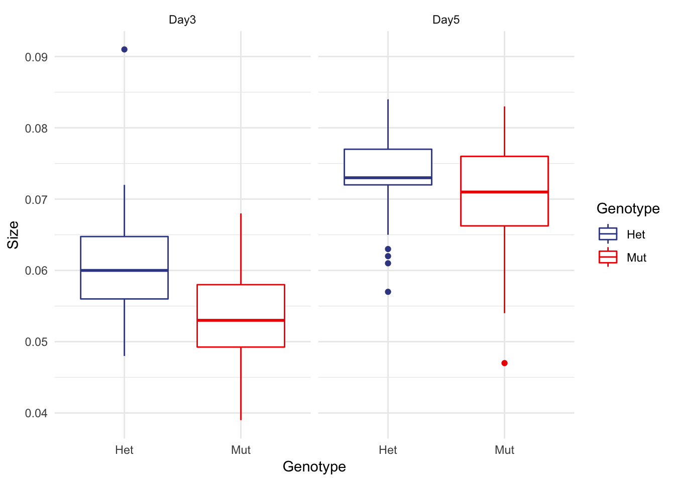
Boxplot with all the data displayed
So easy with ggplot2
Remember to have your geom_boxplot remove display of outliers (since you are showing them now with geom_jitter)
micro %>% ggplot(aes(x=Genotype, y=Size, colour=Genotype)) + facet_wrap(~Date) +
  geom_boxplot(outlier.shape = NA) +
  geom_jitter() +
  theme_minimal() +
  scale_color_aaas()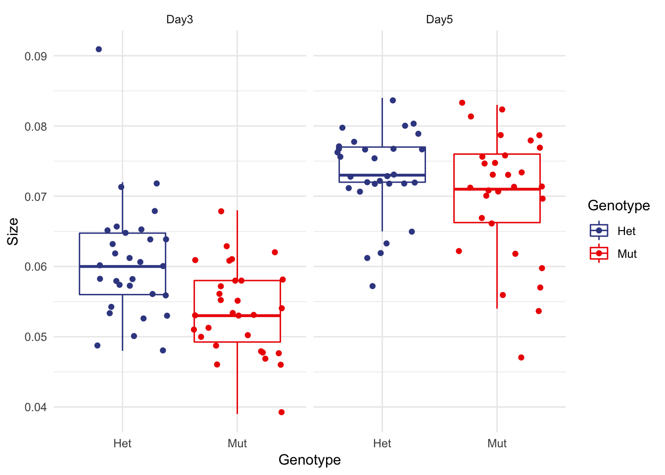
I used to prefer violin plots
But the smoothing for outlier points can be misleading. They also confuse people who haven’t seen them before and you lose the quartile / median info a boxplot provides.
micro %>% ggplot(aes(x=Genotype, y=Size, colour=Genotype)) + facet_wrap(~Date) +
  geom_violin() +
  geom_jitter() +
  theme_minimal() +
  scale_color_aaas()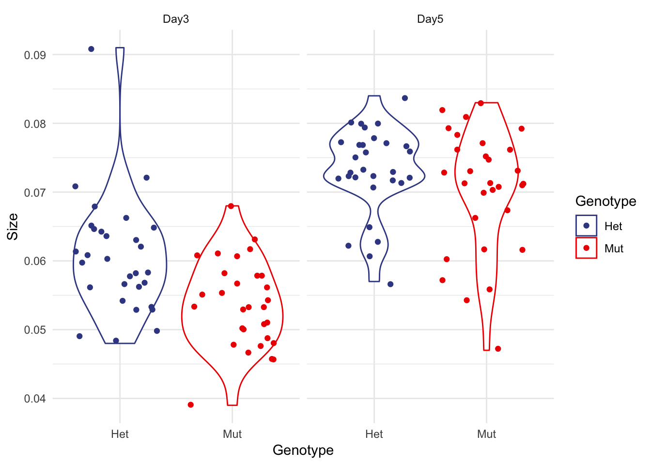
I’m a fan of beeswarm plots with boxplots
You get the violin plot structure and the quartile / median info of boxplots. Win win.
I’ve reduced the alpha (opacity) of the points to put more emphasis on the boxplot.
micro %>% ggplot(aes(x=Genotype, y=Size, colour=Genotype)) + facet_wrap(~Date) +
  geom_boxplot(outlier.shape = NA) +
  geom_quasirandom(alpha=0.4) +
  theme_minimal() +
  scale_color_aaas()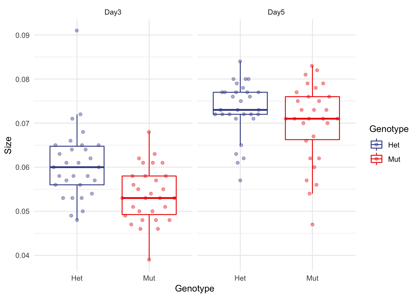
Doing statistics.
Are the differences significant between genotype on Day3 and Day5? More precisely, can we reject the null hypothesis (no mean difference in size)?
Let’s use the venerable t.test. The data eyeballs as normally distributed. I’m using dplyr filter to test Day 3 and Day 5 separately, testing for differences in mean between genotypes (hence the right half of the equation below ends with pull(Genotype))
# Day 3
t.test(micro %>% filter(Date=='Day3') %>% pull(Size) ~ micro %>% filter(Date=='Day3') %>% pull(Genotype))
##
## Welch Two Sample t-test
##
## data: micro %>% filter(Date == "Day3") %>% pull(Size) by micro %>% filter(Date == "Day3") %>% pull(Genotype)
## t = 3.5888, df = 53.629, p-value = 0.0007197
## alternative hypothesis: true difference in means is not equal to 0
## 95 percent confidence interval:
## 0.003029977 0.010703357
## sample estimates:
## mean in group Het mean in group Mut
## 0.06060000 0.05373333# Day 5
t.test(micro %>% filter(Date=='Day5') %>% pull(Size) ~ micro %>% filter(Date=='Day5') %>% pull(Genotype))##
## Welch Two Sample t-test
##
## data: micro %>% filter(Date == "Day5") %>% pull(Size) by micro %>% filter(Date == "Day5") %>% pull(Genotype)
## t = 1.4851, df = 52.164, p-value = 0.1435
## alternative hypothesis: true difference in means is not equal to 0
## 95 percent confidence interval:
## -0.001029920 0.006896587
## sample estimates:
## mean in group Het mean in group Mut
## 0.07313333 0.07020000Yes for Day 3, no for Day 5.
Session
devtools::session_info()## Session info -------------------------------------------------------------## setting value
## version R version 3.5.0 (2018-04-23)
## system x86_64, darwin15.6.0
## ui X11
## language (EN)
## collate en_US.UTF-8
## tz America/New_York
## date 2018-07-16## Packages -----------------------------------------------------------------## package * version date source
## assertthat 0.2.0 2017-04-11 CRAN (R 3.5.0)
## backports 1.1.2 2017-12-13 CRAN (R 3.5.0)
## base * 3.5.0 2018-04-24 local
## beeswarm 0.2.3 2016-04-25 CRAN (R 3.5.0)
## bindr 0.1.1 2018-03-13 CRAN (R 3.5.0)
## bindrcpp * 0.2.2 2018-03-29 CRAN (R 3.5.0)
## blogdown 0.8.1 2018-07-16 Github (rstudio/blogdown@d54c39a)
## bookdown 0.7 2018-02-18 CRAN (R 3.5.0)
## broom 0.4.4 2018-03-29 CRAN (R 3.5.0)
## cellranger 1.1.0 2016-07-27 CRAN (R 3.5.0)
## cli 1.0.0 2017-11-05 CRAN (R 3.5.0)
## colorspace 1.3-2 2016-12-14 CRAN (R 3.5.0)
## compiler 3.5.0 2018-04-24 local
## crayon 1.3.4 2017-09-16 CRAN (R 3.5.0)
## datasets * 3.5.0 2018-04-24 local
## devtools 1.13.5 2018-02-18 CRAN (R 3.5.0)
## digest 0.6.15 2018-01-28 CRAN (R 3.5.0)
## dplyr * 0.7.6 2018-06-29 cran (@0.7.6)
## evaluate 0.10.1 2017-06-24 CRAN (R 3.5.0)
## forcats * 0.3.0 2018-02-19 CRAN (R 3.5.0)
## foreign 0.8-70 2017-11-28 CRAN (R 3.5.0)
## ggbeeswarm * 0.6.0 2017-08-07 CRAN (R 3.5.0)
## ggplot2 * 3.0.0 2018-07-03 cran (@3.0.0)
## ggsci * 2.9 2018-05-14 CRAN (R 3.5.0)
## glue 1.2.0 2017-10-29 CRAN (R 3.5.0)
## graphics * 3.5.0 2018-04-24 local
## grDevices * 3.5.0 2018-04-24 local
## grid 3.5.0 2018-04-24 local
## gtable 0.2.0 2016-02-26 CRAN (R 3.5.0)
## haven 1.1.1 2018-01-18 CRAN (R 3.5.0)
## hms 0.4.2 2018-03-10 CRAN (R 3.5.0)
## htmltools 0.3.6 2017-04-28 CRAN (R 3.5.0)
## httr 1.3.1 2017-08-20 CRAN (R 3.5.0)
## jsonlite 1.5 2017-06-01 CRAN (R 3.5.0)
## knitr 1.20 2018-02-20 CRAN (R 3.5.0)
## labeling 0.3 2014-08-23 CRAN (R 3.5.0)
## lattice 0.20-35 2017-03-25 CRAN (R 3.5.0)
## lazyeval 0.2.1 2017-10-29 CRAN (R 3.5.0)
## lubridate 1.7.4 2018-04-11 CRAN (R 3.5.0)
## magrittr 1.5 2014-11-22 CRAN (R 3.5.0)
## memoise 1.1.0 2017-04-21 CRAN (R 3.5.0)
## methods * 3.5.0 2018-04-24 local
## mnormt 1.5-5 2016-10-15 CRAN (R 3.5.0)
## modelr 0.1.2 2018-05-11 CRAN (R 3.5.0)
## munsell 0.4.3 2016-02-13 CRAN (R 3.5.0)
## nlme 3.1-137 2018-04-07 CRAN (R 3.5.0)
## parallel 3.5.0 2018-04-24 local
## pillar 1.2.3 2018-05-25 CRAN (R 3.5.0)
## pkgconfig 2.0.1 2017-03-21 CRAN (R 3.5.0)
## plyr 1.8.4 2016-06-08 CRAN (R 3.5.0)
## psych 1.8.4 2018-05-06 CRAN (R 3.5.0)
## purrr * 0.2.4 2017-10-18 CRAN (R 3.5.0)
## R6 2.2.2 2017-06-17 CRAN (R 3.5.0)
## Rcpp 0.12.17 2018-05-18 CRAN (R 3.5.0)
## readr * 1.1.1 2017-05-16 CRAN (R 3.5.0)
## readxl 1.1.0 2018-04-20 CRAN (R 3.5.0)
## reshape2 1.4.3 2017-12-11 CRAN (R 3.5.0)
## rlang 0.2.1 2018-05-30 CRAN (R 3.5.0)
## rmarkdown 1.10 2018-06-11 cran (@1.10)
## rprojroot 1.3-2 2018-01-03 CRAN (R 3.5.0)
## rstudioapi 0.7 2017-09-07 CRAN (R 3.5.0)
## rvest 0.3.2 2016-06-17 CRAN (R 3.5.0)
## scales 0.5.0 2017-08-24 CRAN (R 3.5.0)
## stats * 3.5.0 2018-04-24 local
## stringi 1.2.2 2018-05-02 CRAN (R 3.5.0)
## stringr * 1.3.1 2018-05-10 CRAN (R 3.5.0)
## tibble * 1.4.2 2018-01-22 CRAN (R 3.5.0)
## tidyr * 0.8.1 2018-05-18 CRAN (R 3.5.0)
## tidyselect 0.2.4 2018-02-26 CRAN (R 3.5.0)
## tidyverse * 1.2.1 2017-11-14 CRAN (R 3.5.0)
## tools 3.5.0 2018-04-24 local
## utf8 1.1.4 2018-05-24 CRAN (R 3.5.0)
## utils * 3.5.0 2018-04-24 local
## vipor 0.4.5 2017-03-22 CRAN (R 3.5.0)
## withr 2.1.2 2018-03-15 CRAN (R 3.5.0)
## xfun 0.3 2018-07-06 cran (@0.3)
## xml2 1.2.0 2018-01-24 CRAN (R 3.5.0)
## yaml 2.1.19 2018-05-01 CRAN (R 3.5.0)