- Load data
- Curious?
- Data
- How many genes are in this dataset?
- What genes are in here?
- How many data points (bases) per gene?
- How many exons per gene?
- How many base pairs of ABCA4 (well, ABCA4 exons) is covered by more than 10 reads?
- 5 reads?
- Let’s check all of the genes to see which are the worst covered
- We can visually display the data, also
- Hard to see what is going on, let’s make little plots for each gene
- Where are genes poorly covered?
- Make a coverage plot for many genes (This is advanced stuff!!!)
Load data
This is a departure from the previous installments, as we are loading in a very processed dataset. The reasons why are numerous:
- The original data is 330mb, compressed
- After loading (2 minutes on my quite fast computer) and uncompressing, it takes over 10GB of RAM on my computer
- The original data needed a severe amount of massaging to make it quickly useable:
- Annotating with gene name
- Identifying primary transcript for gene
- Expanding range data into row-form*
mosdepthprovides read depth as ranges. So instead of writing a row for each of the three billion+ base pairs,mosdepthcollapses adjacent rows with identical read depth together. This is crucial for saving space, especially for exomes, which have huge stretches of zero coverage since only ~3% of the genome is targeted.
Curious?
If you want to see how I did the above, see Part 2. This post also has some cooler plots.
Data
dd_class.csv can be found here
library(tidyverse)## ── Attaching packages ────────────────────────────────────────────────────────────────────────────────── tidyverse 1.2.1 ──## ✔ ggplot2 3.0.0 ✔ purrr 0.2.5
## ✔ tibble 1.4.2 ✔ dplyr 0.7.6
## ✔ tidyr 0.8.1 ✔ stringr 1.3.1
## ✔ readr 1.1.1 ✔ forcats 0.3.0## ── Conflicts ───────────────────────────────────────────────────────────────────────────────────── tidyverse_conflicts() ──
## ✖ dplyr::filter() masks stats::filter()
## ✖ dplyr::lag() masks stats::lag()library(data.table)##
## Attaching package: 'data.table'## The following objects are masked from 'package:dplyr':
##
## between, first, last## The following object is masked from 'package:purrr':
##
## transposelibrary(cowplot) # you may need to install this with install.packages('cowplot')##
## Attaching package: 'cowplot'## The following object is masked from 'package:ggplot2':
##
## ggsavedd_class <- fread('~/git/Let_us_plot/003_coverage/dd_class.csv')
head(dd_class)## Transcript Exon Number Start Chr End Read_Depth Strand
## 1: ENST00000020945.3 0 49831356 8 49831367 108 -
## 2: ENST00000020945.3 0 49831357 8 49831367 108 -
## 3: ENST00000020945.3 0 49831358 8 49831367 108 -
## 4: ENST00000020945.3 0 49831359 8 49831367 108 -
## 5: ENST00000020945.3 0 49831360 8 49831367 108 -
## 6: ENST00000020945.3 0 49831361 8 49831367 108 -
## ExonStart ExonEnd Name
## 1: 49831365 49831547 SNAI2
## 2: 49831365 49831547 SNAI2
## 3: 49831365 49831547 SNAI2
## 4: 49831365 49831547 SNAI2
## 5: 49831365 49831547 SNAI2
## 6: 49831365 49831547 SNAI2How many genes are in this dataset?
dd_class$Name %>% unique() %>% length()## [1] 118What genes are in here?
dd_class$Name %>% unique() %>% sort()## [1] "ABCA4" "ABCB6" "AIPL1" "ALDH1A3" "ARL6" "ATF6"
## [7] "ATOH7" "BBIP1" "BBS1" "BBS10" "BBS12" "BBS5"
## [13] "BBS7" "BBS9" "BCOR" "BMP4" "CACNA1F" "CACNA2D4"
## [19] "CASK" "CDHR1" "CEP290" "CHD7" "CNGB3" "CNNM4"
## [25] "COL4A1" "COX7B" "CRX" "CYP1B1" "DCDC1" "EDN3"
## [31] "EDNRB" "ELP4" "FKRP" "FKTN" "FOXC1" "FOXC2"
## [37] "FOXE3" "GDF3" "GDF6" "GNAT2" "HESX1" "HMGB3"
## [43] "HPS1" "HPS3" "HPS4" "HPS5" "HPS6" "INPP5E"
## [49] "ISPD" "KCNJ13" "KCNV2" "KIT" "LAMB2" "LHX2"
## [55] "LYST" "LZTFL1" "MAB21L2" "MFRP" "MITF" "MKKS"
## [61] "MKS1" "MLPH" "MYO5A" "NAA10" "NDP" "NPHP1"
## [67] "NRL" "OCA2" "OTX2" "PAX2" "PAX3" "PAX6"
## [73] "PDE6C" "PDE6H" "PITPNM3" "PITX2" "PITX3" "POMT1"
## [79] "POMT2" "PROM1" "PRPH2" "PRSS56" "RAB18" "RAB27A"
## [85] "RAB3GAP1" "RAB3GAP2" "RARB" "RAX" "RAX2" "RDH5"
## [91] "RET" "RIMS1" "RPGR" "RPGRIP1" "SDCCAG8" "SEMA4A"
## [97] "SHH" "SIX3" "SIX6" "SLC24A5" "SLC25A1" "SLC38A8"
## [103] "SLC45A2" "SNAI2" "SNX3" "SOX10" "SOX2" "SOX3"
## [109] "STRA6" "TENM3" "TMEM98" "TRIM32" "TTC8" "TTLL5"
## [115] "UNC119" "VAX1" "VSX2" "ZEB2"How many data points (bases) per gene?
dd_class %>%
  group_by(Name) %>%
  summarise(Count=n())
## # A tibble: 118 x 2
## Name Count
## <chr> <int>
## 1 ABCA4 6804
## 2 ABCB6 2527
## 3 AIPL1 1159
## 4 ALDH1A3 1550
## 5 ARL6 569
## 6 ATF6 2008
## 7 ATOH7 457
## 8 BBIP1 220
## 9 BBS1 1773
## 10 BBS10 2172
## # ... with 108 more rowsHow many exons per gene?
dd_class %>%
  select(Name, `Exon Number`) %>%
  unique() %>%
  group_by(Name) %>%
  summarise(Count = n())
## # A tibble: 118 x 2
## Name Count
## <chr> <int>
## 1 ABCA4 50
## 2 ABCB6 19
## 3 AIPL1 6
## 4 ALDH1A3 13
## 5 ARL6 7
## 6 ATF6 16
## 7 ATOH7 1
## 8 BBIP1 2
## 9 BBS1 17
## 10 BBS10 2
## # ... with 108 more rowsHow many base pairs of ABCA4 (well, ABCA4 exons) is covered by more than 10 reads?
Base R style
# Grab the Read_Depth vector from the data frame filtered by ABCA4 values
depth_abca4 <- dd_class %>%
  filter(Name=='ABCA4') %>%
  pull(Read_Depth)
sum(depth_abca4 > 10)
## [1] 68035 reads?
sum(depth_abca4 > 5)## [1] 6804Let’s check all of the genes to see which are the worst covered
dd_class %>%
  group_by(Name) %>%
  summarise(Total_Bases = n(),
            LT5 = sum(Read_Depth < 5),
            LT10 = sum(Read_Depth < 10),
            Good = sum(Read_Depth >= 10),
            P5 = LT5 / Total_Bases,
            P10 = LT10 / Total_Bases) %>%
  arrange(-P10)
## # A tibble: 118 x 7
## Name Total_Bases LT5 LT10 Good P5 P10
## <chr> <int> <int> <int> <int> <dbl> <dbl>
## 1 BBIP1 220 0 61 159 0 0.277
## 2 ISPD 1339 0 57 1282 0 0.0426
## 3 CASK 2778 0 79 2699 0 0.0284
## 4 NAA10 725 0 10 715 0 0.0138
## 5 CNGB3 2436 0 18 2418 0 0.00739
## 6 LYST 11400 13 66 11334 0.00114 0.00579
## 7 PROM1 2601 0 8 2593 0 0.00308
## 8 RET 3348 0 9 3339 0 0.00269
## 9 CEP290 7456 0 18 7438 0 0.00241
## 10 SLC25A1 933 0 2 931 0 0.00214
## # ... with 108 more rowsWe can visually display the data, also
dd_class %>%
  ggplot(aes(x=Read_Depth, group=Name)) +
  geom_density()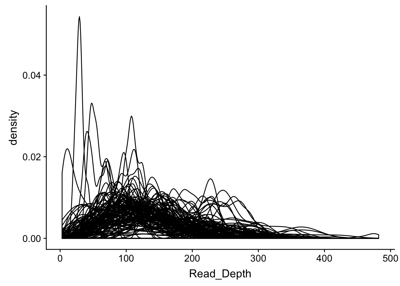
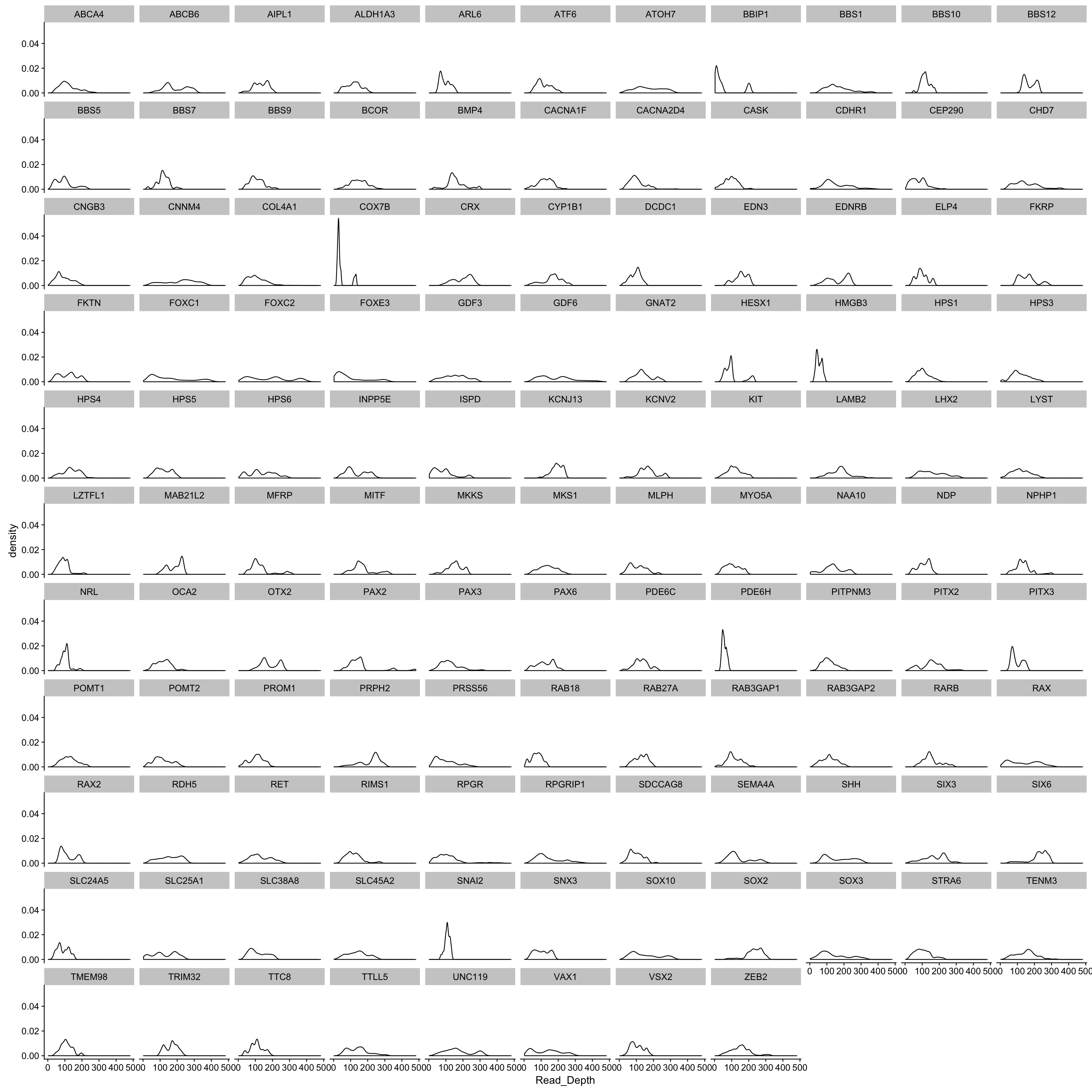
Hard to see what is going on, let’s make little plots for each gene
dd_class %>%
ggplot(aes(x=Read_Depth, group=Name)) +
facet_wrap(~Name) +
geom_density()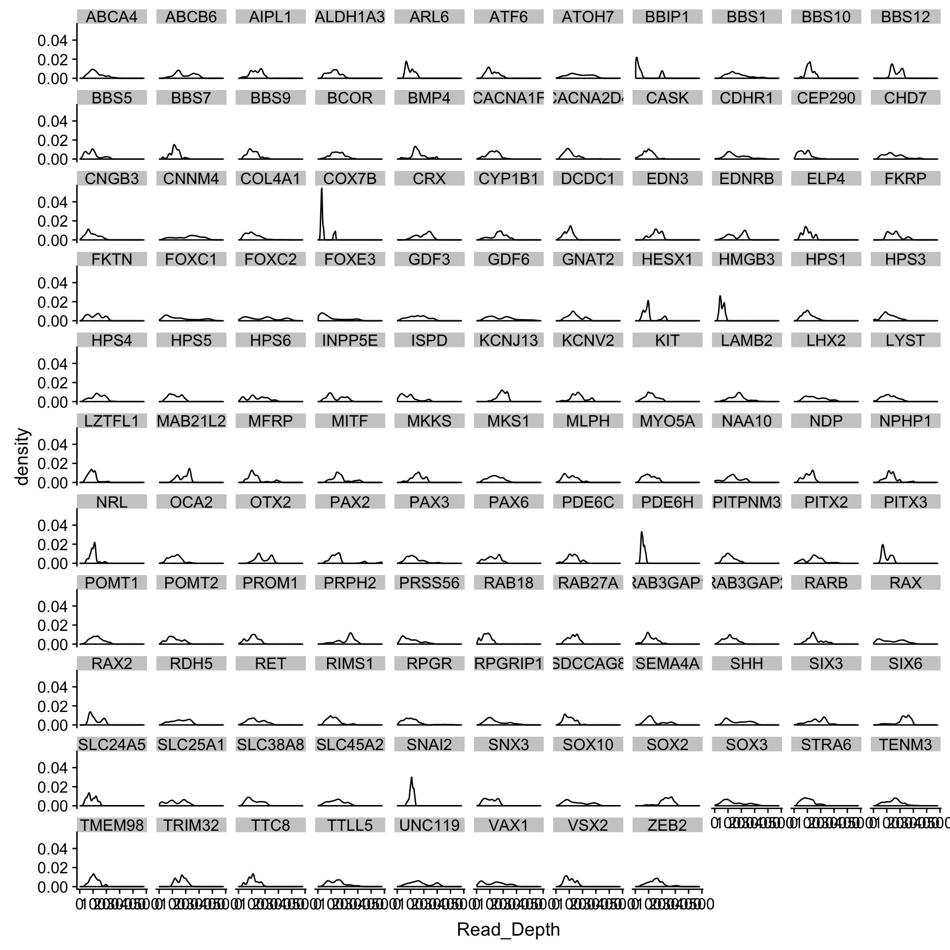 ##
##
Where are genes poorly covered?
BBIP1
dd_class %>% filter(Name=='BBIP1') %>%
  ggplot(aes(x=Start, y=Read_Depth)) +
  facet_wrap(~`Exon Number`, scales = 'free_x', nrow=1, strip.position = 'bottom') +
  geom_point(size=0.1) + theme_minimal() +
  theme(axis.text.x=element_blank(),
        axis.ticks.x = element_blank(),
        panel.grid.minor = element_blank(),
        panel.grid.major.x = element_blank(),
        legend.position = 'none') +
  ylab('Depth') +
  xlab('Exon Number')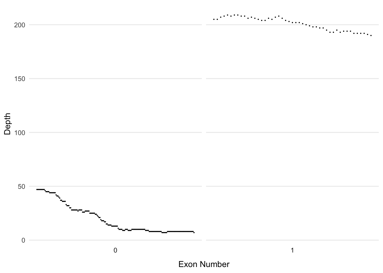
Make a coverage plot for many genes (This is advanced stuff!!!)
gene_list <- c('ABCA4', 'PITX2','VSX2','RPGR','SOX10')

# set a custom color that will work even if a category is missing
scale_colour_custom <- function(...){
  ggplot2:::manual_scale('colour',
                         values = setNames(c('darkred', 'red', 'black'),
                                           c('< 10 Reads','< 20 Reads','>= 20 Reads')),
                         ...)
}

plot_maker <- function(gene){
  num_of_exons <- dd_class%>% filter(Name==gene) %>% pull(`Exon Number`) %>% as.numeric() %>% max()
   # expand to create a row for each sequence and fill in previous values
  dd_class %>% filter(Name==gene) %>%
    mutate(`Exon Number`= factor(`Exon Number`,levels=0:num_of_exons)) %>%
    ggplot(aes(x=Start, y=Read_Depth)) +
    facet_wrap(~`Exon Number`, scales = 'free_x', nrow=1, strip.position = 'bottom') +
    geom_point(size=0.1) + theme_minimal() + scale_colour_custom() +
    theme(axis.text.x=element_blank(),
          axis.ticks.x = element_blank(),
          panel.grid.minor = element_blank(),
          panel.grid.major.x = element_blank(),
          legend.position = 'none') +
    ylab('Depth') +
    xlab(gene)
}

plots <- list()
for (i in gene_list){
  plots[[i]] <- plot_maker(i)
}

plot_grid(plotlist = plots, ncol=1)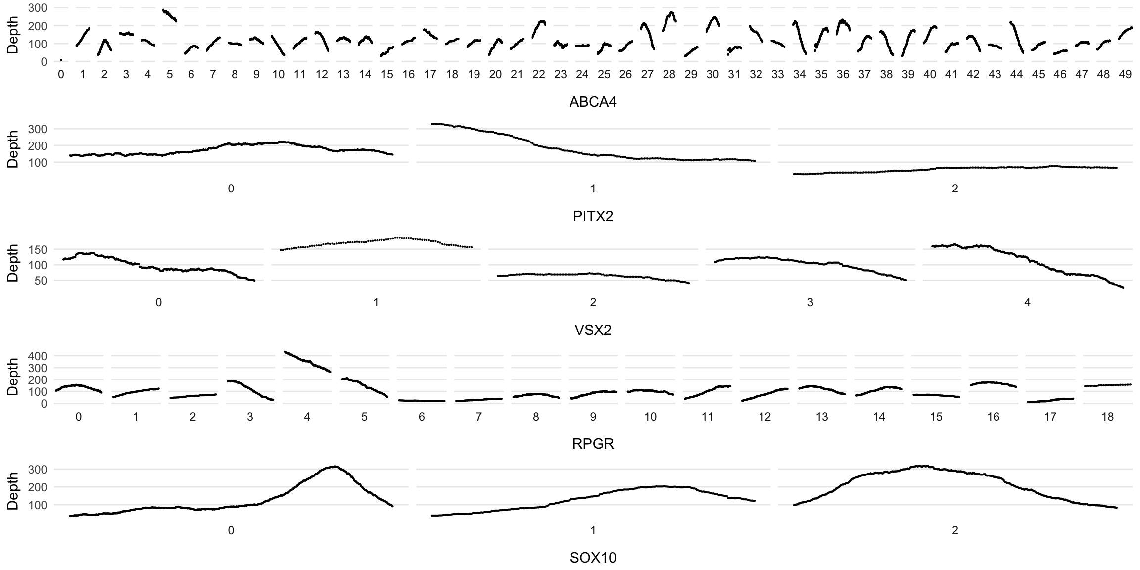
devtools::session_info()## Session info -------------------------------------------------------------## setting value
## version R version 3.5.0 (2018-04-23)
## system x86_64, darwin15.6.0
## ui X11
## language (EN)
## collate en_US.UTF-8
## tz Europe/London
## date 2018-09-17## Packages -----------------------------------------------------------------## package * version date source
## assertthat 0.2.0 2017-04-11 CRAN (R 3.5.0)
## backports 1.1.2 2017-12-13 CRAN (R 3.5.0)
## base * 3.5.0 2018-04-24 local
## bindr 0.1.1 2018-03-13 CRAN (R 3.5.0)
## bindrcpp * 0.2.2 2018-03-29 CRAN (R 3.5.0)
## blogdown 0.8 2018-07-15 CRAN (R 3.5.0)
## bookdown 0.7 2018-02-18 CRAN (R 3.5.0)
## broom 0.4.4 2018-03-29 CRAN (R 3.5.0)
## cellranger 1.1.0 2016-07-27 CRAN (R 3.5.0)
## cli 1.0.0 2017-11-05 CRAN (R 3.5.0)
## colorspace 1.3-2 2016-12-14 CRAN (R 3.5.0)
## compiler 3.5.0 2018-04-24 local
## cowplot * 0.9.3 2018-07-15 cran (@0.9.3)
## crayon 1.3.4 2017-09-16 CRAN (R 3.5.0)
## data.table * 1.11.4 2018-05-27 CRAN (R 3.5.0)
## datasets * 3.5.0 2018-04-24 local
## devtools 1.13.6 2018-06-27 CRAN (R 3.5.0)
## digest 0.6.15 2018-01-28 CRAN (R 3.5.0)
## dplyr * 0.7.6 2018-06-29 cran (@0.7.6)
## evaluate 0.10.1 2017-06-24 CRAN (R 3.5.0)
## forcats * 0.3.0 2018-02-19 CRAN (R 3.5.0)
## foreign 0.8-70 2017-11-28 CRAN (R 3.5.0)
## ggplot2 * 3.0.0 2018-07-03 cran (@3.0.0)
## glue 1.2.0 2017-10-29 CRAN (R 3.5.0)
## graphics * 3.5.0 2018-04-24 local
## grDevices * 3.5.0 2018-04-24 local
## grid 3.5.0 2018-04-24 local
## gtable 0.2.0 2016-02-26 CRAN (R 3.5.0)
## haven 1.1.1 2018-01-18 CRAN (R 3.5.0)
## hms 0.4.2 2018-03-10 CRAN (R 3.5.0)
## htmltools 0.3.6 2017-04-28 CRAN (R 3.5.0)
## httr 1.3.1 2017-08-20 CRAN (R 3.5.0)
## jsonlite 1.5 2017-06-01 CRAN (R 3.5.0)
## knitr 1.20 2018-02-20 CRAN (R 3.5.0)
## labeling 0.3 2014-08-23 CRAN (R 3.5.0)
## lattice 0.20-35 2017-03-25 CRAN (R 3.5.0)
## lazyeval 0.2.1 2017-10-29 CRAN (R 3.5.0)
## lubridate 1.7.4 2018-04-11 CRAN (R 3.5.0)
## magrittr 1.5 2014-11-22 CRAN (R 3.5.0)
## memoise 1.1.0 2017-04-21 CRAN (R 3.5.0)
## methods * 3.5.0 2018-04-24 local
## mnormt 1.5-5 2016-10-15 CRAN (R 3.5.0)
## modelr 0.1.2 2018-05-11 CRAN (R 3.5.0)
## munsell 0.4.3 2016-02-13 CRAN (R 3.5.0)
## nlme 3.1-137 2018-04-07 CRAN (R 3.5.0)
## parallel 3.5.0 2018-04-24 local
## pillar 1.2.3 2018-05-25 CRAN (R 3.5.0)
## pkgconfig 2.0.1 2017-03-21 CRAN (R 3.5.0)
## plyr 1.8.4 2016-06-08 CRAN (R 3.5.0)
## psych 1.8.4 2018-05-06 CRAN (R 3.5.0)
## purrr * 0.2.5 2018-05-29 CRAN (R 3.5.0)
## R6 2.2.2 2017-06-17 CRAN (R 3.5.0)
## Rcpp 0.12.17 2018-05-18 CRAN (R 3.5.0)
## readr * 1.1.1 2017-05-16 CRAN (R 3.5.0)
## readxl 1.1.0 2018-04-20 CRAN (R 3.5.0)
## reshape2 1.4.3 2017-12-11 CRAN (R 3.5.0)
## rlang 0.2.1 2018-05-30 CRAN (R 3.5.0)
## rmarkdown 1.10 2018-06-11 cran (@1.10)
## rprojroot 1.3-2 2018-01-03 CRAN (R 3.5.0)
## rstudioapi 0.7 2017-09-07 CRAN (R 3.5.0)
## rvest 0.3.2 2016-06-17 CRAN (R 3.5.0)
## scales 0.5.0 2017-08-24 CRAN (R 3.5.0)
## stats * 3.5.0 2018-04-24 local
## stringi 1.2.2 2018-05-02 CRAN (R 3.5.0)
## stringr * 1.3.1 2018-05-10 CRAN (R 3.5.0)
## tibble * 1.4.2 2018-01-22 CRAN (R 3.5.0)
## tidyr * 0.8.1 2018-05-18 CRAN (R 3.5.0)
## tidyselect 0.2.4 2018-02-26 CRAN (R 3.5.0)
## tidyverse * 1.2.1 2017-11-14 CRAN (R 3.5.0)
## tools 3.5.0 2018-04-24 local
## utf8 1.1.4 2018-05-24 CRAN (R 3.5.0)
## utils * 3.5.0 2018-04-24 local
## withr 2.1.2 2018-03-15 CRAN (R 3.5.0)
## xfun 0.3 2018-07-06 CRAN (R 3.5.0)
## xml2 1.2.0 2018-01-24 CRAN (R 3.5.0)
## yaml 2.1.19 2018-05-01 CRAN (R 3.5.0)