Build and Apply a Human Brain Region Predictor in 60 seconds or less
2023-07-25
build_a_brain_region_predictor.RmdIntroduction
The GTEx resource contains thousands of human RNA-seq tissues. Here we use the recount3 package to pull the GTEx brain RNA-seq datasets, use a subset to build a brain region predictor, then apply it to the remaining GTEx brain data and bring in a outside human brain study to see whether the model still is useful.
Pull in GTEx brain counts via recount3
This is the longest step in this vignette. Takes me about 10-20 seconds, though your time will vary depending on the vagaries of the internet.
We show the gtex.smtsd to see the brain regions assayed
in GTEx.
library(ggplot2)
library(dplyr)
library(recount3)
# library(metamoRph)
human_projects <- available_projects()

project_info <- subset(human_projects, file_source == "gtex" & project_type == "data_sources" &
    project == "BRAIN")

rse_gene_brain <- create_rse(project_info)

colData(rse_gene_brain)$gtex.smtsd %>%
    table()
#> .
#>                          Brain - Amygdala  Brain - Anterior cingulate cortex (BA24)
#>                                       163                                       201
#>           Brain - Caudate (basal ganglia)             Brain - Cerebellar Hemisphere
#>                                       273                                       250
#>                        Brain - Cerebellum                            Brain - Cortex
#>                                       285                                       286
#>              Brain - Frontal Cortex (BA9)                       Brain - Hippocampus
#>                                       224                                       220
#>                      Brain - Hypothalamus Brain - Nucleus accumbens (basal ganglia)
#>                                       221                                       262
#>           Brain - Putamen (basal ganglia)        Brain - Spinal cord (cervical c-1)
#>                                       221                                       171
#>                  Brain - Substantia nigra
#>                                       154
Extract read counts
brain_counts <- compute_read_counts(rse_gene_brain)Build metadata table for the “train” and “project” data
The train data is used to build the PCA object. That PCA
data is used in the model building. The project data is
then morphed/projected onto the PCA space with metamoRph
and the output from that is used by model_apply to guess
the tissue label.
This all happens in less than 10 seconds on my MacBook.
I find (anecdotally) that using a fairly large number of PC (200 in this case) tends to have modestly label transfer performance with bulk RNA seq data.
set.seed(20230711)
train_meta <- colData(rse_gene_brain) %>%
    as_tibble(rownames = "id") %>%
    group_by(gtex.smtsd) %>%
    sample_n(40)
project_meta <- colData(rse_gene_brain) %>%
    as_tibble(rownames = "id") %>%
    filter(!id %in% train_meta$id)

train_counts <- brain_counts[, train_meta$id]
project_counts <- brain_counts[, project_meta$id]

gtex_pca <- run_pca(train_counts, train_meta)

trained_model <- model_build(gtex_pca$PCA$x, gtex_pca$meta %>%
    pull(gtex.smtsd), num_PCs = 200, verbose = FALSE)

projected_data <- metamoRph(project_counts, gtex_pca$PCA$rotation, gtex_pca$center_scale)
# apply model
label_guesses <- model_apply(trained_model, projected_data, project_meta %>%
pull(gtex.smtsd))Visualizing the label outcomes on the PC
You can see how in many of the “misablels” are on the edge (or further!) of the groups.
bind_rows(projected_data %>%
    as_tibble(rownames = "id")) %>%
    left_join(colData(rse_gene_brain) %>%
        as_tibble(rownames = "id"), by = "id") %>%
    left_join(label_guesses, by = c(id = "sample_id")) %>%
    mutate(correct = case_when(sample_label == predict ~ "Yes", TRUE ~ "No")) %>%
    ggplot(aes(x = PC1, y = PC2, color = correct)) + geom_point(alpha = 0.5) + cowplot::theme_cowplot() +
    facet_wrap(~gtex.smtsd)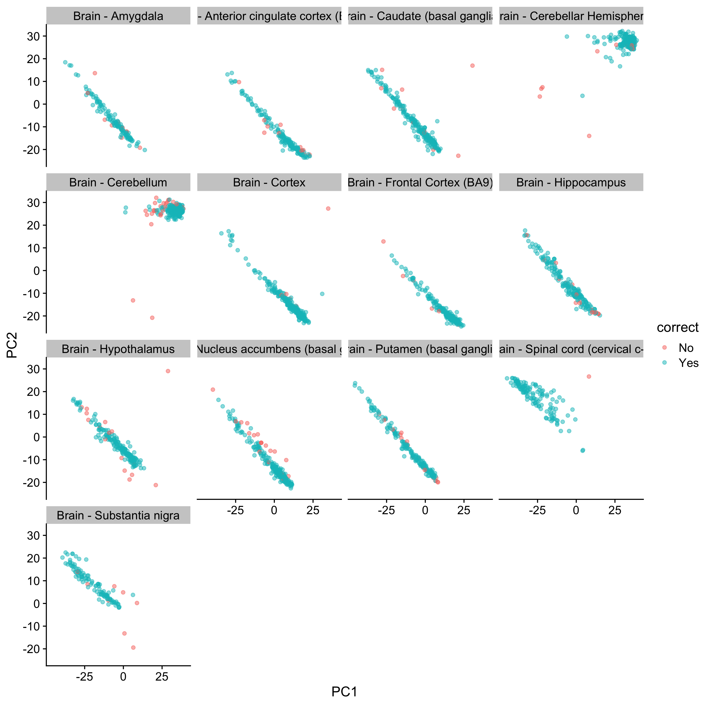
Now a harder thing - using outside data on the model we built
BA9 prefontal cortex - and the model built still has ~89% accuracy.
# outside brain prefrontal cortex (BA9)
outside_gtex <- subset(human_projects, project_type == "data_sources" & project == "SRP058181")
rse_gene_outside <- create_rse(outside_gtex)

outside_counts <- compute_read_counts(rse_gene_outside)
outside_meta <- colData(rse_gene_outside) %>%
    as_tibble(rownames = "id")
outside_counts <- outside_counts[, outside_meta$id]


projected_data_outside <- metamoRph(outside_counts, gtex_pca$PCA$rotation, gtex_pca$center_scale)
label_guesses_outside <- model_apply(trained_model, projected_data_outside)Session Info
sessionInfo()
#> R version 4.3.0 (2023-04-21)
#> Platform: aarch64-apple-darwin20 (64-bit)
#> Running under: macOS Ventura 13.4.1
#>
#> Matrix products: default
#> BLAS:   /System/Library/Frameworks/Accelerate.framework/Versions/A/Frameworks/vecLib.framework/Versions/A/libBLAS.dylib
#> LAPACK: /Library/Frameworks/R.framework/Versions/4.3-arm64/Resources/lib/libRlapack.dylib;  LAPACK version 3.11.0
#>
#> locale:
#> [1] en_US.UTF-8/en_US.UTF-8/en_US.UTF-8/C/en_US.UTF-8/en_US.UTF-8
#>
#> time zone: America/New_York
#> tzcode source: internal
#>
#> attached base packages:
#> [1] stats4    stats     graphics  grDevices utils     datasets  methods   base
#>
#> other attached packages:
#>  [1] tictoc_1.2                  metamoRph_0.2.0             testthat_3.1.8
#>  [4] projectR_1.16.0             recount3_1.10.2             SummarizedExperiment_1.30.1
#>  [7] Biobase_2.60.0              GenomicRanges_1.52.0        GenomeInfoDb_1.36.0
#> [10] IRanges_2.34.0              S4Vectors_0.38.1            BiocGenerics_0.46.0
#> [13] MatrixGenerics_1.12.0       matrixStats_0.63.0          knitr_1.43
#> [16] scMerge_1.16.0              patchwork_1.1.2             cowplot_1.1.1
#> [19] ggplot2_3.4.2               uwot_0.1.14                 Matrix_1.5-4.1
#> [22] dplyr_1.1.2                 panc8.SeuratData_3.0.2      SeuratData_0.2.2
#> [25] SeuratObject_4.1.3          Seurat_4.3.0.1
#>
#> loaded via a namespace (and not attached):
#>   [1] R.methodsS3_1.8.2           dichromat_2.0-0.1           progress_1.2.2
#>   [4] urlchecker_1.0.1            nnet_7.3-19                 goftest_1.2-3
#>   [7] Biostrings_2.67.2           rstan_2.21.8                vctrs_0.6.2
#>  [10] spatstat.random_3.1-5       digest_0.6.31               png_0.1-8
#>  [13] registry_0.5-1              ggrepel_0.9.3               deldir_1.0-9
#>  [16] parallelly_1.36.0           batchelor_1.15.1            MASS_7.3-60
#>  [19] pkgdown_2.0.7               reshape2_1.4.4              foreach_1.5.2
#>  [22] httpuv_1.6.11               withr_2.5.0                 xfun_0.39
#>  [25] ellipsis_0.3.2              survival_3.5-5              commonmark_1.9.0
#>  [28] memoise_2.0.1               proxyC_0.3.3                rcmdcheck_1.4.0
#>  [31] ggbeeswarm_0.7.2            profvis_0.3.8               zoo_1.8-12
#>  [34] gtools_3.9.4                pbapply_1.7-2               R.oo_1.25.0
#>  [37] DEoptimR_1.1-0              Formula_1.2-5               prettyunits_1.1.1
#>  [40] KEGGREST_1.39.0             promises_1.2.0.1            httr_1.4.6
#>  [43] restfulr_0.0.15             rhdf5filters_1.12.1         globals_0.16.2
#>  [46] fitdistrplus_1.1-11         cvTools_0.3.2               rhdf5_2.44.0
#>  [49] ps_1.7.5                    rstudioapi_0.14             miniUI_0.1.1.1
#>  [52] generics_0.1.3              ggalluvial_0.12.5           base64enc_0.1-3
#>  [55] processx_3.8.1              babelgene_22.9              curl_5.0.0
#>  [58] zlibbioc_1.46.0             sfsmisc_1.1-15              ScaledMatrix_1.8.1
#>  [61] polyclip_1.10-4             xopen_1.0.0                 GenomeInfoDbData_1.2.10
#>  [64] doParallel_1.0.17           xtable_1.8-4                stringr_1.5.0
#>  [67] desc_1.4.2                  evaluate_0.21               S4Arrays_1.0.4
#>  [70] BiocFileCache_2.7.2         hms_1.1.3                   irlba_2.3.5.1
#>  [73] colorspace_2.1-0            filelock_1.0.2              ROCR_1.0-11
#>  [76] CoGAPS_3.19.1               reticulate_1.28             spatstat.data_3.0-1
#>  [79] magrittr_2.0.3              lmtest_0.9-40               later_1.3.1
#>  [82] viridis_0.6.3               lattice_0.21-8              mapproj_1.2.11
#>  [85] NMF_0.26                    spatstat.geom_3.2-2         future.apply_1.11.0
#>  [88] robustbase_0.99-0           scattermore_1.1             XML_3.99-0.14
#>  [91] scuttle_1.9.4               RcppAnnoy_0.0.20            Hmisc_5.1-0
#>  [94] pillar_1.9.0                StanHeaders_2.26.27         nlme_3.1-162
#>  [97] iterators_1.0.14            gridBase_0.4-7              caTools_1.18.2
#> [100] compiler_4.3.0              beachmat_2.15.0             stringi_1.7.12
#> [103] tensor_1.5                  devtools_2.4.5              GenomicAlignments_1.35.1
#> [106] plyr_1.8.8                  msigdbr_7.5.1               crayon_1.5.2
#> [109] abind_1.4-5                 BiocIO_1.9.2                scater_1.28.0
#> [112] locfit_1.5-9.7              pals_1.7                    sp_2.0-0
#> [115] waldo_0.5.1                 bit_4.0.5                   fastmatch_1.1-3
#> [118] codetools_0.2-19            BiocSingular_1.15.0         bslib_0.5.0
#> [121] plotly_4.10.1               mime_0.12                   splines_4.3.0
#> [124] Rcpp_1.0.10                 dbplyr_2.3.2                sparseMatrixStats_1.11.1
#> [127] blob_1.2.4                  utf8_1.2.3                  reldist_1.7-2
#> [130] fs_1.6.2                    listenv_0.9.0               checkmate_2.2.0
#> [133] DelayedMatrixStats_1.21.0   pkgbuild_1.4.0              tibble_3.2.1
#> [136] callr_3.7.3                 statmod_1.5.0               tweenr_2.0.2
#> [139] startupmsg_0.9.6            pkgconfig_2.0.3             tools_4.3.0
#> [142] cachem_1.0.8                RSQLite_2.3.1               viridisLite_0.4.2
#> [145] DBI_1.1.3                   numDeriv_2016.8-1.1         fastmap_1.1.1
#> [148] rmarkdown_2.21              scales_1.2.1                grid_4.3.0
#> [151] usethis_2.1.6               ica_1.0-3                   Rsamtools_2.15.2
#> [154] sass_0.4.6                  BiocManager_1.30.20         RANN_2.6.1
#> [157] rpart_4.1.19                farver_2.1.1                mgcv_1.8-42
#> [160] yaml_2.3.7                  roxygen2_7.2.3              foreign_0.8-84
#> [163] rtracklayer_1.59.1          cli_3.6.1                   purrr_1.0.1
#> [166] leiden_0.4.3                lifecycle_1.0.3             M3Drop_1.26.0
#> [169] mvtnorm_1.1-3               bluster_1.9.1               sessioninfo_1.2.2
#> [172] backports_1.4.1             BiocParallel_1.33.11        distr_2.9.2
#> [175] gtable_0.3.3                rjson_0.2.21                ggridges_0.5.4
#> [178] densEstBayes_1.0-2.2        progressr_0.13.0            parallel_4.3.0
#> [181] limma_3.56.1                jsonlite_1.8.4              edgeR_3.42.2
#> [184] bitops_1.0-7                bit64_4.0.5                 brio_1.1.3
#> [187] Rtsne_0.16                  spatstat.utils_3.0-3        BiocNeighbors_1.17.1
#> [190] RcppParallel_5.1.7          bdsmatrix_1.3-6             jquerylib_0.1.4
#> [193] highr_0.10                  metapod_1.7.0               dqrng_0.3.0
#> [196] loo_2.6.0                   R.utils_2.12.2              lazyeval_0.2.2
#> [199] shiny_1.7.4                 ruv_0.9.7.1                 htmltools_0.5.5
#> [202] sctransform_0.3.5           rappdirs_0.3.3              formatR_1.14
#> [205] glue_1.6.2                  ResidualMatrix_1.10.0       XVector_0.40.0
#> [208] RCurl_1.98-1.12             rprojroot_2.0.3             scran_1.27.1
#> [211] gridExtra_2.3               igraph_1.4.3                R6_2.5.1
#> [214] tidyr_1.3.0                 SingleCellExperiment_1.22.0 gplots_3.1.3
#> [217] forcats_1.0.0               labeling_0.4.2              rngtools_1.5.2
#> [220] cluster_2.1.4               bbmle_1.0.25                Rhdf5lib_1.22.0
#> [223] pkgload_1.3.2               rstantools_2.3.1            DelayedArray_0.26.6
#> [226] tidyselect_1.2.0            vipor_0.4.5                 htmlTable_2.4.1
#> [229] maps_3.4.1                  ggforce_0.4.1               xml2_1.3.4
#> [232] inline_0.3.19               AnnotationDbi_1.61.2        future_1.32.0
#> [235] rsvd_1.0.5                  munsell_0.5.0               KernSmooth_2.23-21
#> [238] data.table_1.14.8           fgsea_1.25.0                htmlwidgets_1.6.2
#> [241] RColorBrewer_1.1-3          biomaRt_2.55.0              rlang_1.1.1
#> [244] spatstat.sparse_3.0-2       spatstat.explore_3.2-1      remotes_2.4.2
#> [247] fansi_1.0.4                 beeswarm_0.4.0