Batch Corrected metamoRph Reference
2023-07-25
dataset_integration_and_projection.RmdMotivation
You want to build a batch corrected scRNA-seq reference from several disparate datasets to use as a resource for label transfer and visualization onto new data.
So…
metamoRph is not a batch correction tool. Just a small set of functions to enable projection of data onto an existing reference resource.
Using a disparate set of scRNA datasets with
metamoRph::run_pca requires those datasets to be batch
corrected.
Here we present two approaches: one using Seurat’s
IntegrateData and another with scMerge2 to generate
corrected counts.
To demonstrate that the applicability of metamoRph can extend beyond data I am cherry picking from the variety of ocular resources I have curated, we will use the data from Seurat’s Mapping and annotating query datasets guide.
Why not just use Seurat the whole way through?????
Seurat has a very full set of tools to do just about everything - including the batch correction, projecting new data onto it, and then transfer the labels and make a matching UMAP. The code that does that is reproduced in the first code chunk.
Why even bother using metamoRph? There are two reasons. First, is that metamoRph is a general projection engine. You can use it for bulk RNA. You can use it for scRNA. There is no reason why you can’t use it for other kinds of information! PCA (or SVD) are tremendous dimensionality reduction approaches and I find it amazing that, with a touch of attention about data preprocessing, you can project (morph!) new data onto an existing PCA space with just a matrix multiplication. The second is speed. Because our approach is so simple, once you have built a reference, you can morph new data and do the label transfer in second(s).
Why can’t I use the PCA I already made with Seurat?
Unfortunately you can’t use the Seurat PCA because they do not return
the center and scaling values used in their internal data normalization.
The bog standard prcomp function does return these
values, so if the PCA you are using is from prcomp (or
inspired by prcomp) then those values can be extracted from
the returned object with
metamoRph::extract_prcomp_scaling().
Seurat Dataset Integration
This code is taken from the Seurat v4 Mapping and annotating query datasets guide. The git link to the guide is here, should the previous link go dead or the guide is substantially changed in the future.
Integrate
data("panc8")

pancreas.list <- SplitObject(panc8, split.by = "tech")
pancreas.list <- pancreas.list[c("celseq", "celseq2", "fluidigmc1", "smartseq2")]

tictoc::tic()
for (i in 1:length(pancreas.list)) {
    pancreas.list[[i]] <- NormalizeData(pancreas.list[[i]], verbose = FALSE)
    pancreas.list[[i]] <- FindVariableFeatures(pancreas.list[[i]], selection.method = "vst", nfeatures = 2000,
        verbose = FALSE)
}


reference.list <- pancreas.list[c("celseq", "celseq2", "smartseq2")]
pancreas.anchors <- FindIntegrationAnchors(object.list = reference.list, dims = 1:30)

pancreas.integrated <- IntegrateData(anchorset = pancreas.anchors, dims = 1:30)
seurat_integration_timing <- tictoc::toc()
Map New Data Onto Reference
Seurat’s approach results in 617 correct labels and 21 incorrect. Given the UMAP viz (cue Lior Pachter screaming) probably a few of those “incorrect” are mislabels.
tictoc::tic()
# switch to integrated assay. The variable features of this assay are automatically set during
# IntegrateData
DefaultAssay(pancreas.integrated) <- "integrated"
# Run the standard workflow for visualization and clustering
pancreas.integrated <- ScaleData(pancreas.integrated, verbose = FALSE)
pancreas.integrated <- RunPCA(pancreas.integrated, npcs = 30, verbose = FALSE)
pancreas.integrated <- RunUMAP(pancreas.integrated, reduction = "pca", dims = 1:30, verbose = FALSE)
seurat_rebuild_analysis_on_corrected_data_timing <- tictoc::toc()
#> 11.549 sec elapsed
# p1 <- DimPlot(pancreas.integrated, reduction = 'umap', group.by = 'tech') p2 <-
# DimPlot(pancreas.integrated, reduction = 'umap', group.by = 'celltype', label = TRUE, repel
# = TRUE) + NoLegend() p1 + p2

tictoc::tic()

# project new data onto reference and build matching umap
pancreas.query <- pancreas.list[["fluidigmc1"]]
pancreas.anchors <- FindTransferAnchors(reference = pancreas.integrated, query = pancreas.query,
    dims = 1:30, reference.reduction = "pca")
predictions <- TransferData(anchorset = pancreas.anchors, refdata = pancreas.integrated$celltype,
    dims = 1:30)
pancreas.query <- AddMetaData(pancreas.query, metadata = predictions)

pancreas.integrated <- RunUMAP(pancreas.integrated, dims = 1:30, reduction = "pca", return.model = TRUE)
pancreas.query <- MapQuery(anchorset = pancreas.anchors, reference = pancreas.integrated, query = pancreas.query,
    refdata = list(celltype = "celltype"), reference.reduction = "pca", reduction.model = "umap")

pancreas.query$prediction.match <- pancreas.query$predicted.id == pancreas.query$celltype
table(pancreas.query$prediction.match)
#>
#> FALSE  TRUE
#>    21   617
seurat_default_accuracy <- sum(pancreas.query$prediction.match)/length(pancreas.query$prediction.match)

# end timing BEFOFE the plotting step so we don't also compare plotting efficiency
seurat_projection_timing <- tictoc::toc()
#> 15.34 sec elapsed

p1 <- DimPlot(pancreas.integrated, reduction = "umap", group.by = "celltype", label = TRUE, label.size = 3,
    repel = TRUE) + NoLegend() + ggtitle("Reference annotations")
p2 <- DimPlot(pancreas.query, reduction = "ref.umap", group.by = "predicted.celltype", label = TRUE,
    label.size = 3, repel = TRUE) + NoLegend() + ggtitle("Query transferred labels")


p1 + p2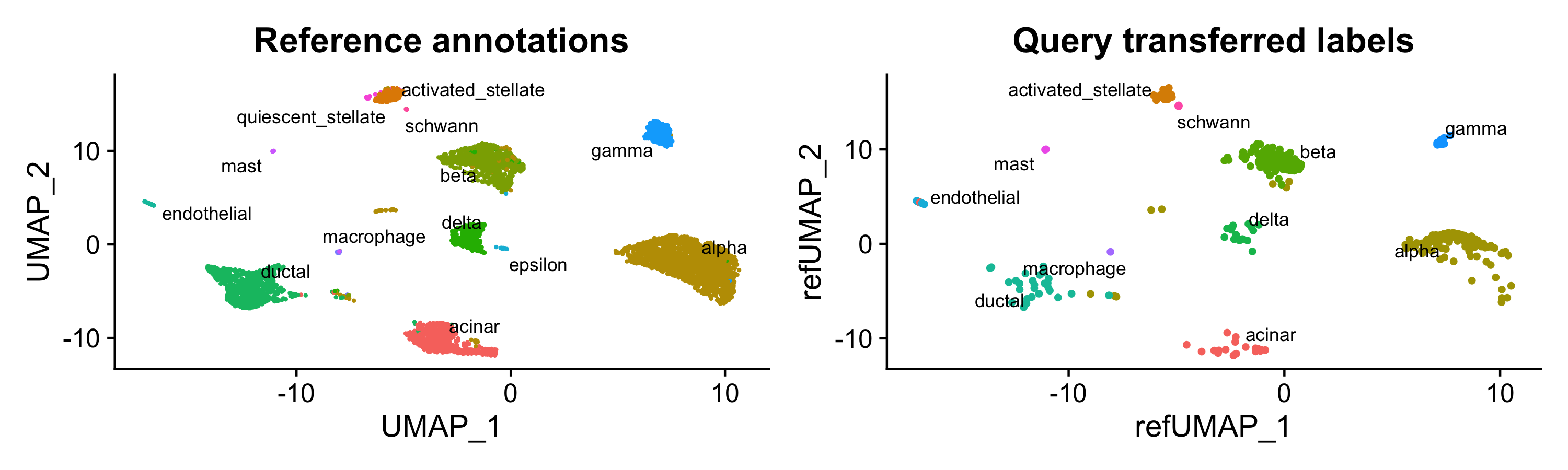
Leverage Seurat’s Corrected Counts in metamoRph
The first approach we demonstrate is to directly use Seurat’s corrected counts from the code chunk above in building a “metamoRph” reference and then projecting/morphing the new data onto it. Read the commented lines in the code block to see explanations of why certain parameters were used in metamoRph.
tictoc::tic()

# here we pull the corrected counts from the `integrated` slot and use it as the reference
# data NOTE 1: see how we have TURNED OFF NORMALIZATION as the data already is normalized NOTE
# 2: we have changed ntop from the default of 1000 to 2000 to match what Seurat uses in their
# example
reference_obj <- metamoRph::run_pca(as.matrix(pancreas.integrated@assays$integrated@data), meta = pancreas.integrated@meta.data,
    method = "irlba", normalization = FALSE, irlba_n = 30, ntop = 2000)
# Seurat and scran both use cosine instead of euclidean as the metric see also how we have the
# full umap model returned this is required downstream
ref_umap <- uwot::umap(reference_obj$PCA$x[, 1:30], metric = "cosine", ret_model = TRUE)
metamoRph_build_ref_from_seurat_counts <- tictoc::toc()
#> 8.702 sec elapsed

# plotting code first we are going to stick some of the first lines into a little function to
# reduce copy/pasting for the later plots

quick_plotter <- function(umap_data, matching_metadata, point_color = "celltype") {
    matching_metadata$group <- matching_metadata[, point_color]
    umap_data %>%
        as_tibble(rownames = "bc") %>%
        left_join(matching_metadata %>%
            as_tibble(rownames = "bc")) %>%
        ggplot(aes(x = V1, y = V2, color = group)) + geom_point(size = 1) + ggrepel::geom_text_repel(data = . %>%
        group_by(group) %>%
        summarise(V1 = mean(V1), V2 = mean(V2)), aes(label = group, color = group), alpha = 0.9,
        bg.color = "white") + cowplot::theme_cowplot() + xlab("") + ylab("") + scale_color_manual(values = pals::glasbey() %>%
        unname()) + theme(legend.position = "none")
}
a <- quick_plotter(ref_umap$embedding, pancreas.integrated@meta.data, "celltype") + ggtitle("Reference: celseq, celseq2, smartseq2")
tictoc::tic()

# here is where we take the new/query data `pancreas.query` and yank out the raw counts we
# specify that metamoRph should transform the counts data using the 'Seurat' approach instead
# of the default 'cpm' approach
query_morphed <- metamoRph::metamoRph(as.matrix(pancreas.query@assays$RNA@counts), reference_obj$PCA$rotation[,
    1:30], center_scale = reference_obj$center_scale, sample_scale = "seurat")
# now we use the reference data PCA ($PCA$x slot) in our model builder to build a cell type
# label guesser from the known labels 'reference_obj$meta$celltype'
ml <- metamoRph::model_build(reference_obj$PCA$x[, 1:30], reference_obj$meta$celltype)
# now we use the models we built to apply to the new data's metamoRph projected PCA space
ma <- metamoRph::model_apply(ml, query_morphed, pancreas.query@meta.data$celltype)

seurat_metamorph_accuracy <- ma %>%
    filter(sample_label == predict) %>%
    nrow()/ma %>%
    filter(!is.na(sample_label)) %>%
    nrow()
paste("Accuracy:", seurat_metamorph_accuracy)
#> [1] "Accuracy: 0.946708463949843"

paste("# Correct:", ma %>%
    filter(sample_label == predict) %>%
    nrow())
#> [1] "# Correct: 604"
paste("# Wrong:", ma %>%
    filter(sample_label != predict) %>%
    nrow())
#> [1] "# Wrong: 34"


umap_proj <- umap_transform(query_morphed[, 1:30], ref_umap)

seurat_metamorph_project_timing <- tictoc::toc()
#> 0.747 sec elapsed

b <- quick_plotter(umap_proj, pancreas.query@meta.data, "celltype") + ggtitle("Query: fluidigmc1")


cowplot::plot_grid(a, b)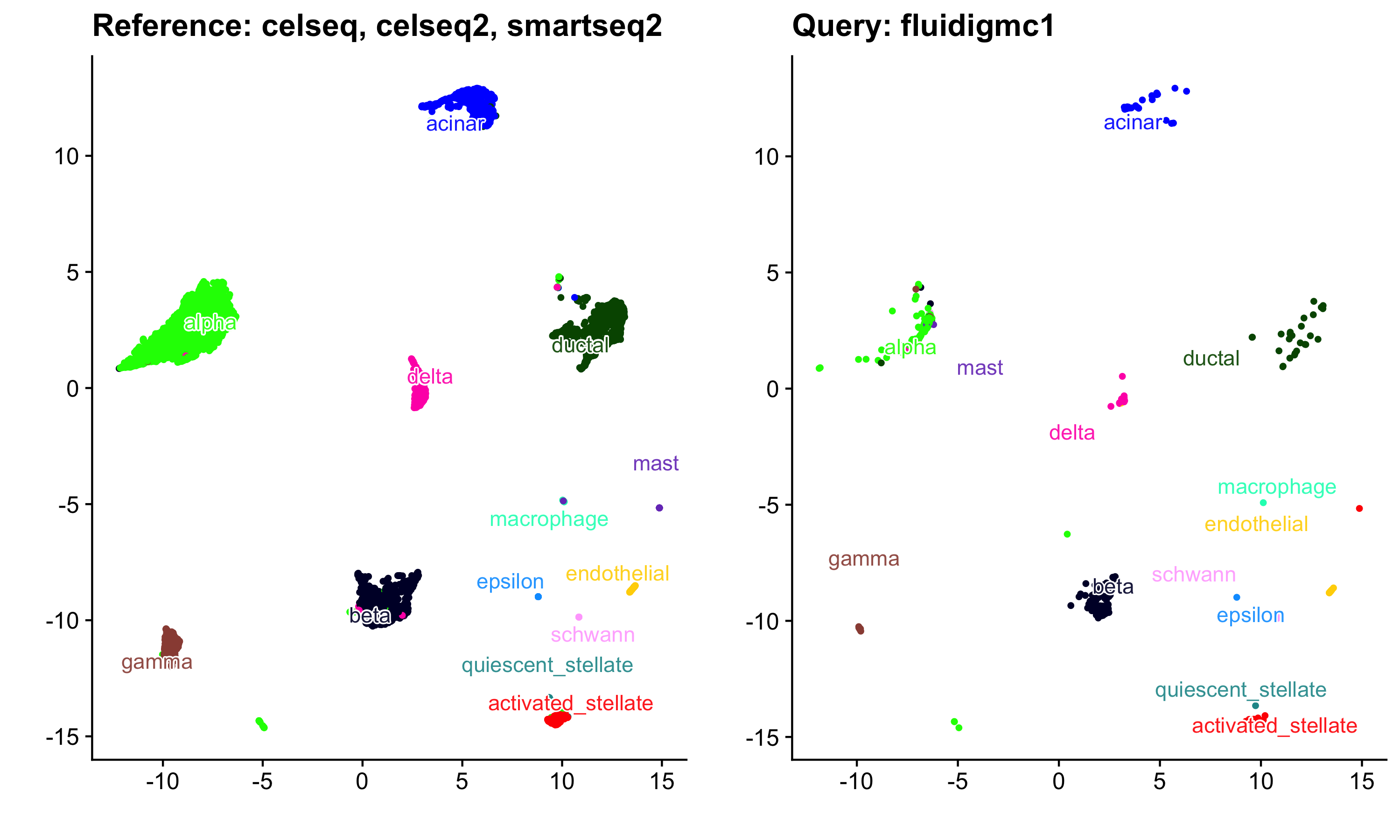
scMerge2 Batch Correction as Input to metamoRph
This is a different approach then before. Here Seurat is not used at
all. Instead we give the raw counts to
metamoRph::normalize_data which is used internally by
metamoRph::run_pca to library and log1p normalize the
counts as required by scMerge2.
We find the top 2000 HVG and feed this matrix into scMerge2 to generate
batch correct counts. We use this batch corrected counts to build our
metamoRph PCA reference, then project/morph the new data on it. We use
the projected/morphed PCA space to make a new UMAP and move labels over,
as we have done earlier.
# metaMorph
tictoc::tic()
# cpm and log1p norm the data
dat <- metamoRph::normalize_data(cbind(pancreas.list[[1]]@assays$RNA@counts, pancreas.list[[2]]@assays$RNA@counts,
    pancreas.list[[3]]@assays$RNA@counts))

meta <- rbind(pancreas.list[[1]]@meta.data, pancreas.list[[2]]@meta.data, pancreas.list[[3]]@meta.data)
# identify the top 2000 HVG
hvg_genes <- metamoRph::select_HVG(dat, ntop = 2000)
# make corrected expression matrix Note: we turn off the unneeded cosineNorm
scmerge_correction <- scMerge2(dat[hvg_genes, ], batch = meta$tech, cosineNorm = FALSE, cellTypes = meta$celltype,
    verbose = FALSE, seed = "2023.0723")
# pull corrected matrix out of the scmerge2 object
corrected_dat <- scmerge_correction$newY %>%
    as.matrix()
# again we turn off normalization as the scmerge corrected data has already been cpm and log1p
# normalized
scmerge2_batch_cor_timing <- tictoc::toc()
#> 11.978 sec elapsed

tictoc::tic()
reference_obj <- metamoRph::run_pca(corrected_dat, meta = meta, method = "irlba", irlba_n = 30,
    normalization = FALSE, ntop = 2000)


# run umap
ref_umap_scMerge2 <- uwot::umap(as.matrix(reference_obj$PCA$x[, 1:30]), metric = "cosine", ret_model = TRUE)
metamoRph_ref_with_scmerge2_correct_counts <- tictoc::toc()
#> 5.986 sec elapsed
a <- quick_plotter(ref_umap_scMerge2$embedding, reference_obj$meta, "celltype") + ggtitle("Reference: celseq, celseq2, smartseq2")
# create projected PCA space with the new data via metamoRph's matrix multplication

tictoc::tic()
query_morphed <- metamoRph::metamoRph(as.matrix(pancreas.query@assays$RNA@counts), reference_obj$PCA$rotation[,
    1:30], center_scale = reference_obj$center_scale)


# build cell type label model
ml <- metamoRph::model_build(as.matrix(reference_obj$PCA$x[, 1:30]), meta$celltype)
# apply the model
ma <- metamoRph::model_apply(ml, query_morphed, pancreas.query@meta.data$celltype)

scmerge2_metamorph_accuracy <- ma %>%
    filter(sample_label == predict) %>%
    nrow()/ma %>%
    filter(!is.na(sample_label)) %>%
    nrow()
paste("Accuracy:", scmerge2_metamorph_accuracy)
#> [1] "Accuracy: 0.970219435736677"
paste("# Correct:", ma %>%
    filter(sample_label == predict) %>%
    nrow())
#> [1] "# Correct: 619"
paste("# Wrong:", ma %>%
    filter(sample_label != predict) %>%
    nrow())
#> [1] "# Wrong: 19"

# project the morphed PCA space of the new data onto the existing PCA we built above
umap_proj <- umap_transform(query_morphed[, 1:30], ref_umap_scMerge2)

b <- quick_plotter(umap_proj, pancreas.query@meta.data, "celltype") + ggtitle("Query: fluidigmc1")


cowplot::plot_grid(a, b)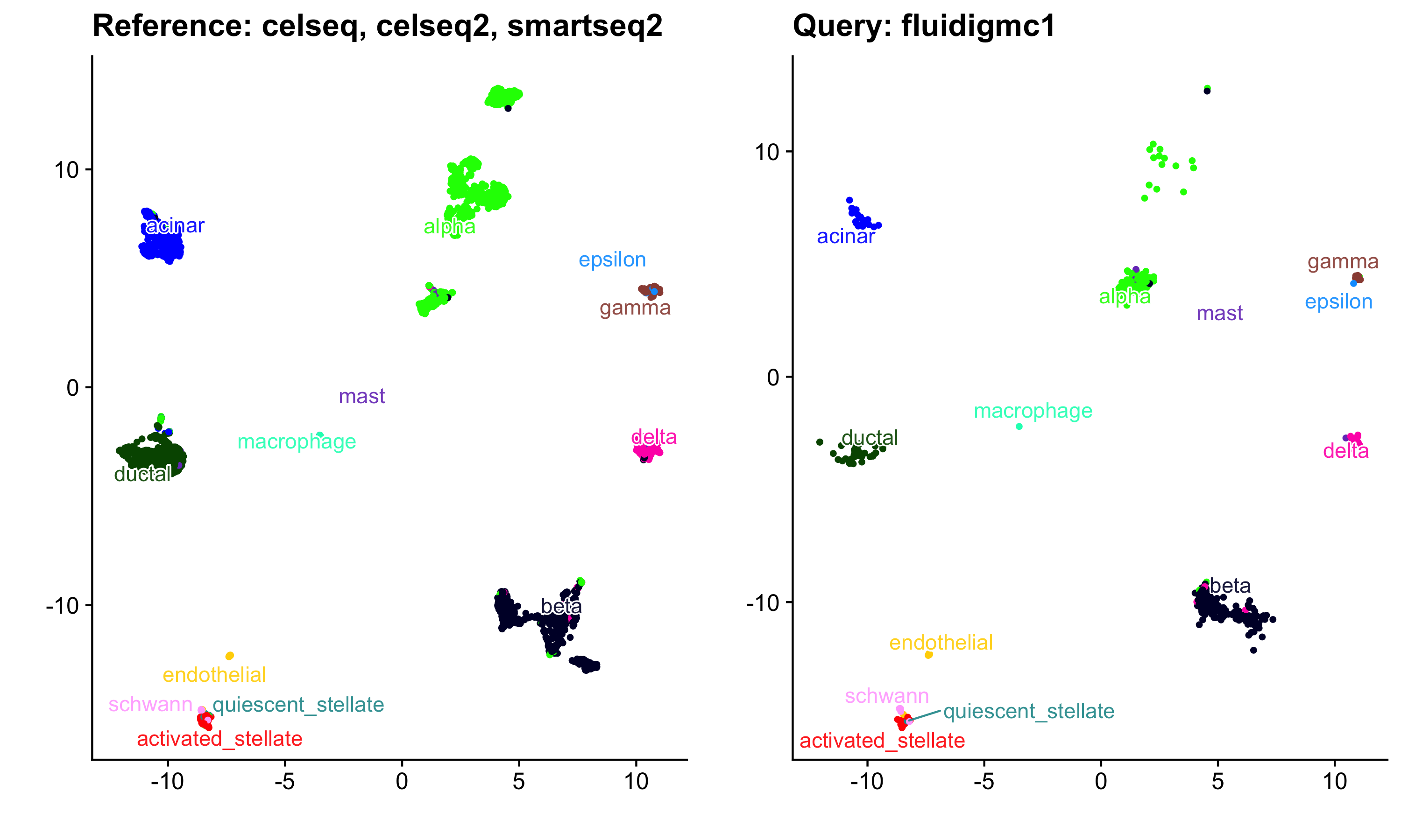
metamorph_scmerge2_morph_timing <- tictoc::toc()
#> 1.023 sec elapsed
Timings
Full Seurat is the slowest approach.
metamoRph IS NOT A BATCH CORRECTION tool and thus there is nothing to record in the “Batch Correction” category for metamoRph.
Building the reference data in Seurat or metamoRph is about the same time. The slowest step is identical between the two - the irlba PCA/SVD dimensionality reduction.
Projecting the new data onto the reference is about 20x faster in metamoRph compared to Seurat.
batch_correction_timing <- c(substr(seurat_integration_timing$callback_msg, 1, 4) %>%
    as.numeric(), substr(scmerge2_batch_cor_timing$callback_msg, 1, 4) %>%
    as.numeric())
names(batch_correction_timing) <- c("Seurat", "scMerge2")

build_reference <- c(substr(seurat_rebuild_analysis_on_corrected_data_timing$callback_msg, 1, 4) %>%
    as.numeric(), substr(metamoRph_build_ref_from_seurat_counts$callback_msg, 1, 4) %>%
    as.numeric(), substr(metamoRph_ref_with_scmerge2_correct_counts$callback_msg, 1, 4) %>%
    as.numeric())

names(build_reference) <- c("Seurat", "metamoRph (Seurat origin)", "metamoRph (scMerge2 origin)")

projection_timing <- c(substr(seurat_projection_timing$callback_msg, 1, 4) %>%
    as.numeric(), substr(seurat_metamorph_project_timing$callback_msg, 1, 4) %>%
    as.numeric(), substr(metamorph_scmerge2_morph_timing$callback_msg, 1, 4) %>%
    as.numeric())
names(projection_timing) <- c("Seurat", "metamoRph (Seurat origin)", "metamoRph (scMerge2 origin)")


bind_rows(data.frame(batch_correction_timing) %>%
    as_tibble(rownames = "Method") %>%
    mutate(Step = "Batch Correction") %>%
    dplyr::rename(time = batch_correction_timing), data.frame(build_reference) %>%
    as_tibble(rownames = "Method") %>%
    mutate(Step = "Build Reference") %>%
    dplyr::rename(time = build_reference), data.frame(projection_timing) %>%
    as_tibble(rownames = "Method") %>%
    mutate(Step = "Query Projection") %>%
    dplyr::rename(time = projection_timing)) %>%
    mutate(Method = factor(Method, levels = c("Seurat", "metamoRph*", "scMerge2", "metamoRph (Seurat origin)",
        "metamoRph (scMerge2 origin)") %>%
        rev())) %>%
    ggplot(aes(y = Method, x = time)) + geom_bar(stat = "identity") + facet_wrap(~Step, scales = "free_y") +
    xlab("Time (seconds)") + geom_text(aes(label = time), hjust = "inward", color = "orange", size = 6) +
    cowplot::theme_cowplot()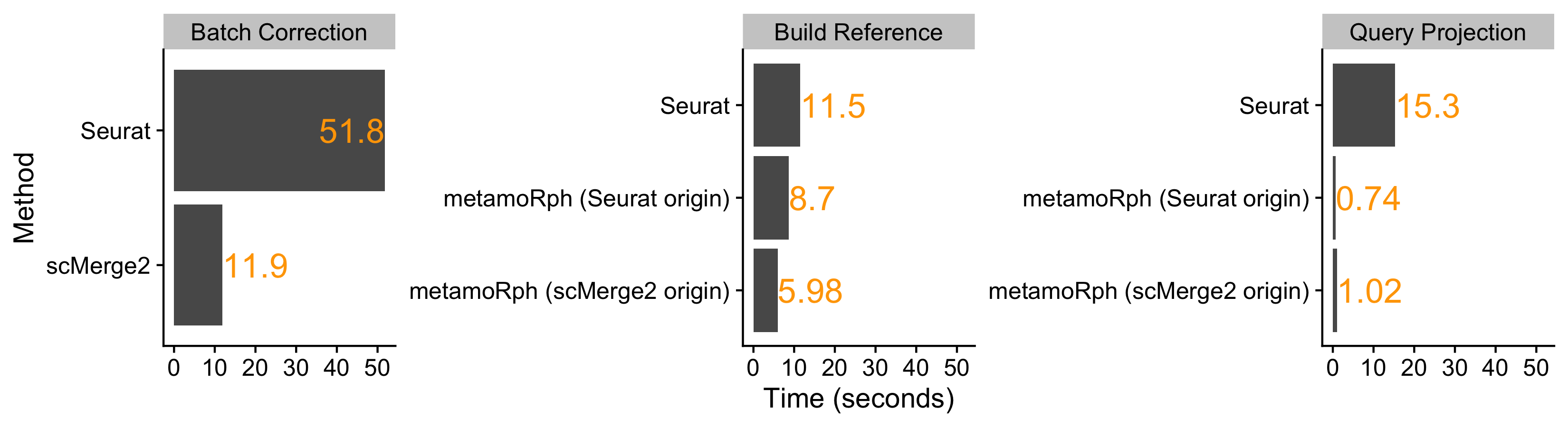
Accuracy of Label Transfer
All three approaches have highly similar accuracy. I guess if you are getting really nit picky the Seurat counts used in metamoRph are a touch worse than full Seurat and the scMerge2/Seurat approach is a bit better. But all work pretty well in my opinion.
accuracy <- c(seurat_default_accuracy, seurat_metamorph_accuracy, scmerge2_metamorph_accuracy) %>%
    data.frame()
accuracy$method <- c("Seurat", "metamoRph (Seurat origin)", "metamoRph (scMerge2 origin)")
colnames(accuracy) <- c("Accuracy", "Method")
accuracy %>%
    mutate(Accuracy = Accuracy * 100) %>%
    ggplot(aes(y = Method, x = Accuracy)) + geom_bar(stat = "identity") + geom_text(aes(label = round(Accuracy,
    2)), hjust = "inward", color = "orange", size = 6) + cowplot::theme_cowplot() + ylab("Method") +
    xlab("% Correct Transferred Cell Type Labels") + coord_cartesian(xlim = c(0, 100))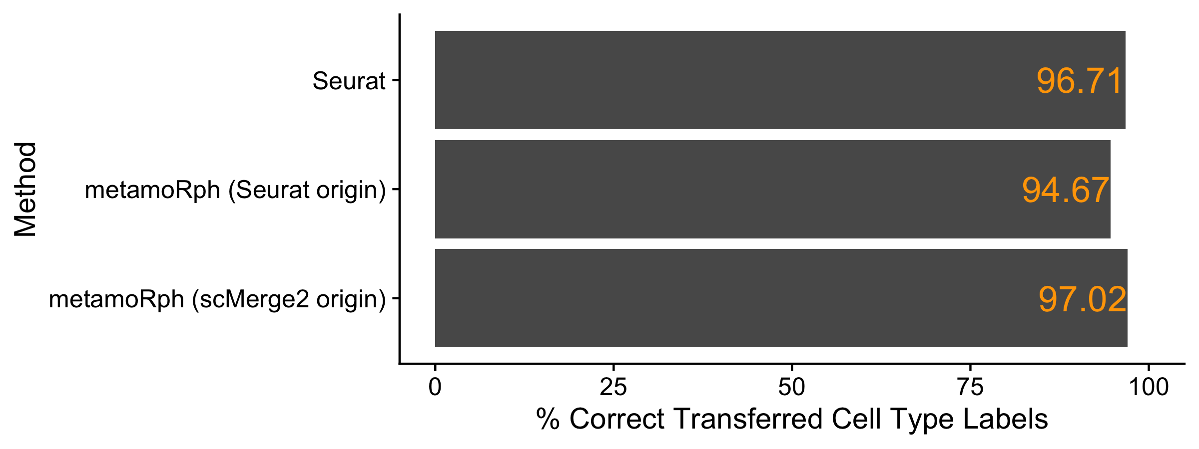
Session Info
sessionInfo()
#> R version 4.3.0 (2023-04-21)
#> Platform: aarch64-apple-darwin20 (64-bit)
#> Running under: macOS Ventura 13.4.1
#>
#> Matrix products: default
#> BLAS:   /System/Library/Frameworks/Accelerate.framework/Versions/A/Frameworks/vecLib.framework/Versions/A/libBLAS.dylib
#> LAPACK: /Library/Frameworks/R.framework/Versions/4.3-arm64/Resources/lib/libRlapack.dylib;  LAPACK version 3.11.0
#>
#> locale:
#> [1] en_US.UTF-8/en_US.UTF-8/en_US.UTF-8/C/en_US.UTF-8/en_US.UTF-8
#>
#> time zone: America/New_York
#> tzcode source: internal
#>
#> attached base packages:
#> [1] stats4    stats     graphics  grDevices utils     datasets  methods   base
#>
#> other attached packages:
#>  [1] tictoc_1.2                  metamoRph_0.2.0             testthat_3.1.8
#>  [4] projectR_1.16.0             recount3_1.10.2             SummarizedExperiment_1.30.1
#>  [7] Biobase_2.60.0              GenomicRanges_1.52.0        GenomeInfoDb_1.36.0
#> [10] IRanges_2.34.0              S4Vectors_0.38.1            BiocGenerics_0.46.0
#> [13] MatrixGenerics_1.12.0       matrixStats_0.63.0          knitr_1.43
#> [16] scMerge_1.16.0              patchwork_1.1.2             cowplot_1.1.1
#> [19] ggplot2_3.4.2               uwot_0.1.14                 Matrix_1.5-4.1
#> [22] dplyr_1.1.2                 panc8.SeuratData_3.0.2      SeuratData_0.2.2
#> [25] SeuratObject_4.1.3          Seurat_4.3.0.1
#>
#> loaded via a namespace (and not attached):
#>   [1] R.methodsS3_1.8.2           dichromat_2.0-0.1           progress_1.2.2
#>   [4] urlchecker_1.0.1            nnet_7.3-19                 goftest_1.2-3
#>   [7] Biostrings_2.67.2           rstan_2.21.8                vctrs_0.6.2
#>  [10] spatstat.random_3.1-5       digest_0.6.31               png_0.1-8
#>  [13] registry_0.5-1              ggrepel_0.9.3               deldir_1.0-9
#>  [16] parallelly_1.36.0           batchelor_1.15.1            MASS_7.3-60
#>  [19] pkgdown_2.0.7               reshape2_1.4.4              foreach_1.5.2
#>  [22] httpuv_1.6.11               withr_2.5.0                 xfun_0.39
#>  [25] ellipsis_0.3.2              survival_3.5-5              commonmark_1.9.0
#>  [28] memoise_2.0.1               proxyC_0.3.3                rcmdcheck_1.4.0
#>  [31] ggbeeswarm_0.7.2            profvis_0.3.8               zoo_1.8-12
#>  [34] gtools_3.9.4                pbapply_1.7-2               R.oo_1.25.0
#>  [37] DEoptimR_1.1-0              Formula_1.2-5               prettyunits_1.1.1
#>  [40] KEGGREST_1.39.0             promises_1.2.0.1            httr_1.4.6
#>  [43] restfulr_0.0.15             rhdf5filters_1.12.1         globals_0.16.2
#>  [46] fitdistrplus_1.1-11         cvTools_0.3.2               rhdf5_2.44.0
#>  [49] ps_1.7.5                    rstudioapi_0.14             miniUI_0.1.1.1
#>  [52] generics_0.1.3              ggalluvial_0.12.5           base64enc_0.1-3
#>  [55] processx_3.8.1              babelgene_22.9              curl_5.0.0
#>  [58] zlibbioc_1.46.0             sfsmisc_1.1-15              ScaledMatrix_1.8.1
#>  [61] polyclip_1.10-4             xopen_1.0.0                 GenomeInfoDbData_1.2.10
#>  [64] doParallel_1.0.17           xtable_1.8-4                stringr_1.5.0
#>  [67] desc_1.4.2                  evaluate_0.21               S4Arrays_1.0.4
#>  [70] BiocFileCache_2.7.2         hms_1.1.3                   irlba_2.3.5.1
#>  [73] colorspace_2.1-0            filelock_1.0.2              ROCR_1.0-11
#>  [76] CoGAPS_3.19.1               reticulate_1.28             spatstat.data_3.0-1
#>  [79] magrittr_2.0.3              lmtest_0.9-40               later_1.3.1
#>  [82] viridis_0.6.3               lattice_0.21-8              mapproj_1.2.11
#>  [85] NMF_0.26                    spatstat.geom_3.2-2         future.apply_1.11.0
#>  [88] robustbase_0.99-0           scattermore_1.1             XML_3.99-0.14
#>  [91] scuttle_1.9.4               RcppAnnoy_0.0.20            Hmisc_5.1-0
#>  [94] pillar_1.9.0                StanHeaders_2.26.27         nlme_3.1-162
#>  [97] iterators_1.0.14            gridBase_0.4-7              caTools_1.18.2
#> [100] compiler_4.3.0              beachmat_2.15.0             stringi_1.7.12
#> [103] tensor_1.5                  devtools_2.4.5              GenomicAlignments_1.35.1
#> [106] plyr_1.8.8                  msigdbr_7.5.1               crayon_1.5.2
#> [109] abind_1.4-5                 BiocIO_1.9.2                scater_1.28.0
#> [112] locfit_1.5-9.7              pals_1.7                    sp_2.0-0
#> [115] waldo_0.5.1                 bit_4.0.5                   fastmatch_1.1-3
#> [118] codetools_0.2-19            BiocSingular_1.15.0         bslib_0.5.0
#> [121] plotly_4.10.1               mime_0.12                   splines_4.3.0
#> [124] Rcpp_1.0.10                 dbplyr_2.3.2                sparseMatrixStats_1.11.1
#> [127] blob_1.2.4                  utf8_1.2.3                  reldist_1.7-2
#> [130] fs_1.6.2                    listenv_0.9.0               checkmate_2.2.0
#> [133] DelayedMatrixStats_1.21.0   pkgbuild_1.4.0              tibble_3.2.1
#> [136] callr_3.7.3                 statmod_1.5.0               tweenr_2.0.2
#> [139] startupmsg_0.9.6            pkgconfig_2.0.3             tools_4.3.0
#> [142] cachem_1.0.8                RSQLite_2.3.1               viridisLite_0.4.2
#> [145] DBI_1.1.3                   numDeriv_2016.8-1.1         fastmap_1.1.1
#> [148] rmarkdown_2.21              scales_1.2.1                grid_4.3.0
#> [151] usethis_2.1.6               ica_1.0-3                   Rsamtools_2.15.2
#> [154] sass_0.4.6                  BiocManager_1.30.20         RANN_2.6.1
#> [157] rpart_4.1.19                farver_2.1.1                mgcv_1.8-42
#> [160] yaml_2.3.7                  roxygen2_7.2.3              foreign_0.8-84
#> [163] rtracklayer_1.59.1          cli_3.6.1                   purrr_1.0.1
#> [166] leiden_0.4.3                lifecycle_1.0.3             M3Drop_1.26.0
#> [169] mvtnorm_1.1-3               bluster_1.9.1               sessioninfo_1.2.2
#> [172] backports_1.4.1             BiocParallel_1.33.11        distr_2.9.2
#> [175] gtable_0.3.3                rjson_0.2.21                ggridges_0.5.4
#> [178] densEstBayes_1.0-2.2        progressr_0.13.0            parallel_4.3.0
#> [181] limma_3.56.1                jsonlite_1.8.4              edgeR_3.42.2
#> [184] bitops_1.0-7                bit64_4.0.5                 brio_1.1.3
#> [187] Rtsne_0.16                  spatstat.utils_3.0-3        BiocNeighbors_1.17.1
#> [190] RcppParallel_5.1.7          bdsmatrix_1.3-6             jquerylib_0.1.4
#> [193] highr_0.10                  metapod_1.7.0               dqrng_0.3.0
#> [196] loo_2.6.0                   R.utils_2.12.2              lazyeval_0.2.2
#> [199] shiny_1.7.4                 ruv_0.9.7.1                 htmltools_0.5.5
#> [202] sctransform_0.3.5           rappdirs_0.3.3              formatR_1.14
#> [205] glue_1.6.2                  ResidualMatrix_1.10.0       XVector_0.40.0
#> [208] RCurl_1.98-1.12             rprojroot_2.0.3             scran_1.27.1
#> [211] gridExtra_2.3               igraph_1.4.3                R6_2.5.1
#> [214] tidyr_1.3.0                 SingleCellExperiment_1.22.0 gplots_3.1.3
#> [217] forcats_1.0.0               labeling_0.4.2              rngtools_1.5.2
#> [220] cluster_2.1.4               bbmle_1.0.25                Rhdf5lib_1.22.0
#> [223] pkgload_1.3.2               rstantools_2.3.1            DelayedArray_0.26.6
#> [226] tidyselect_1.2.0            vipor_0.4.5                 htmlTable_2.4.1
#> [229] maps_3.4.1                  ggforce_0.4.1               xml2_1.3.4
#> [232] inline_0.3.19               AnnotationDbi_1.61.2        future_1.32.0
#> [235] rsvd_1.0.5                  munsell_0.5.0               KernSmooth_2.23-21
#> [238] data.table_1.14.8           fgsea_1.25.0                htmlwidgets_1.6.2
#> [241] RColorBrewer_1.1-3          biomaRt_2.55.0              rlang_1.1.1
#> [244] spatstat.sparse_3.0-2       spatstat.explore_3.2-1      remotes_2.4.2
#> [247] fansi_1.0.4                 beeswarm_0.4.0