Transfer Labels from a Retina scRNA Reference onto a Query Dataset

2023-07-25

Introduction

When we discuss data projection (or morphing! branding!), we have two primary kinds of data. First, the reference, which has been previously analyzed and labelled. Second is the query, which is new data that you wish to speed up your understanding of by transferring knowledge (like cell type or tissue label) from the reference.

metamoRph

This package has four primary functions:

metamoRph::run_pca

This takes in raw count data, matched meta data, and outputs a list object containing a prcomp object and some extra information: percent standard deviation explained by each PC, a center_scale list which has the center and scale values calculated in prcomp and are needed to properly normalize the query data, the meta data itself, and finally the parameters given to metamoRph::run_pca

library(Seurat)
# library(metamoRph)
library(dplyr)
library(uwot)
library(ggplot2)
tictoc::tic()
# download:
# https://hpc.nih.gov/~mcgaugheyd/scEiaD/2021_11_11/study_level/SRP255195.seurat.Rdata
load("~/Downloads/SRP255195.seurat.Rdata")
reference <- scEiaD  # these objects from the plae resource are named 'scEiaD' so we should rename it right away

#### filter down to cell types with at least 50 cells
reference_meta <- reference@meta.data %>%
    as_tibble(rownames = "bc")
set.seed(2023.0721)
celltypes_to_keep <- reference_meta %>%
    group_by(CellType_predict) %>%
    summarise(Count = n()) %>%
    filter(Count >= 50, !is.na(CellType_predict)) %>%
    pull(CellType_predict)
reference_meta <- reference_meta %>%
    filter(CellType_predict %in% celltypes_to_keep)

######## cut down reference matrix to the well represented cell types
ref_mat <- reference@assays$RNA@counts[, reference_meta$bc]

#
mm_pca <- metamoRph::run_pca(feature_by_sample = ref_mat, meta = reference_meta, method = "irlba",
    irlba_n = 50)

Diversion

You can put these principal components (store in mm_pca$PCA$x) into UMAP to make a dangerous (distance has little meaning!) but useful visualization

umap_reference <- uwot::umap(rbind(mm_pca$PCA$x[, 1:20]), ret_model = TRUE)


man_color <- pals::glasbey()
names(man_color) <- celltypes_to_keep %>%
    sort()


ref_viz <- umap_reference$embedding %>%
    as_tibble(rownames = "bc") %>%
    left_join(bind_rows(reference@meta.data %>%
        as_tibble(rownames = "bc"), new_data@meta.data %>%
        as_tibble(rownames = "bc"))) %>%
    ggplot(aes(x = V1, y = V2, color = CellType_predict)) + geom_point(size = 0, alpha = 0.2) +
    cowplot::theme_cowplot() + xlab("") + ylab("") + scale_color_manual(values = man_color) + ggrepel::geom_text_repel(data = . %>%
    group_by(CellType_predict) %>%
    summarise(V1 = mean(V1), V2 = mean(V2)), aes(label = CellType_predict), bg.color = "white") +
    theme(legend.position = "none") + ggtitle("Reference: SRP255195")
ref_viz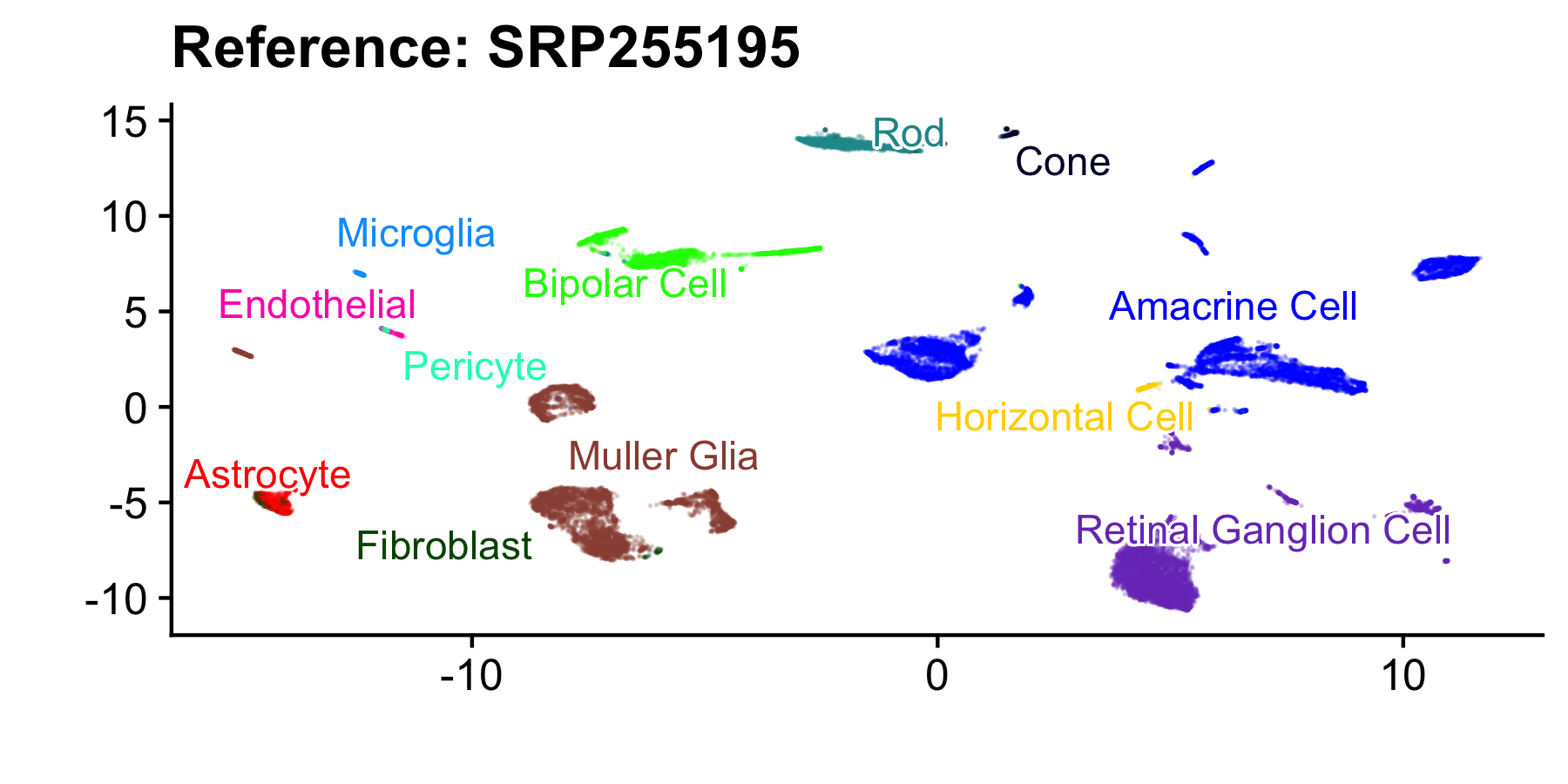

plot of chunk retina scRNA transfer labels first umap

metamoRph::metamoRph

This takes the rotation matrix (prcomp’s $rotation) and center/scale values calculated in metamoRph::run_pca and the query (the new) data as input. The query data features (genes) are matched to the reference data, normalized in the same manner as the reference data, then multiplied against the rotation matrix. This creates a sample by PCA space which can be directly compared with the PCA of the reference data.

# https://hpc.nih.gov/~mcgaugheyd/scEiaD/2021_11_11/study_level/E-MTAB-7316.seurat.Rdata
load("~/Downloads/E-MTAB-7316.seurat.Rdata")
new_data <- scEiaD
pmat <- new_data@assays$RNA@counts
proj <- metamoRph(new_counts = pmat, rotation = mm_pca$PCA$rotation[, 1:50], center_scale = mm_pca$center_scale)

umap_new_data <- umap_transform(proj[, 1:20], umap_reference)


b <- umap_new_data %>%
    as_tibble(rownames = "bc") %>%
    left_join(bind_rows(reference@meta.data %>%
        as_tibble(rownames = "bc"), new_data@meta.data %>%
        as_tibble(rownames = "bc"))) %>%
    filter(!is.na(CellType_predict), CellType_predict %in% celltypes_to_keep) %>%
    ggplot(aes(x = V1, y = V2, color = CellType_predict)) + scattermore::geom_scattermore(pointsize = 2) +
    cowplot::theme_cowplot() + xlab("") + ylab("") + scale_color_manual(values = man_color) + ggrepel::geom_label_repel(data = . %>%
    group_by(CellType_predict) %>%
    summarise(V1 = mean(V1), V2 = mean(V2)), aes(label = CellType_predict), alpha = 0.9) + theme(legend.position = "none") +
    ggtitle("Morphed: EMTAB7316")


cowplot::plot_grid(a, b, ncol = 2, align = "v", axis = "r")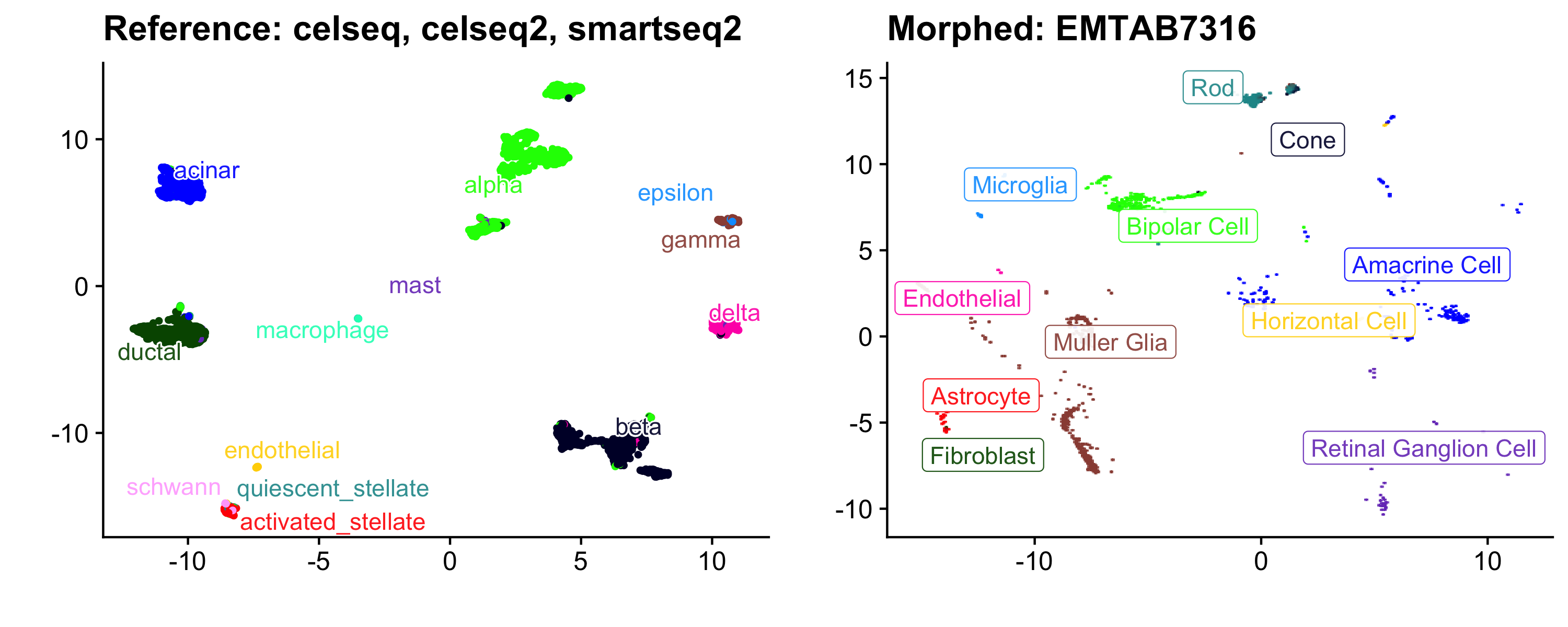

plot of chunk retina scRNA transfer labels comparison umap

Label Transfer via ML

metamoRph::model_build

metamoRph also can perform label transfer (that’s the meta in metamoRph) with metamoRph::model_build. It trains a linear regression for each unique entry in the metadata field. So if you have seven cell types, it will train seven models which are tuned to distinguish each cell type against all remaining data.

You may be wondering why I’m using something as simple as a linear regression. Model build does support different models. Right now it also can use random forest, xgboost, glm, and svm. In practice I suggest the linear regression (“lr”) as it reliably performs the best and is the fastest option. SVM is a pretty close second. I have also experimented with several neural network based models and as they all perform substantially worse, I chose not to make them available.

metamoRph::model_apply

metamoRph::model_build returns a list object with a model trained for each unique field (in this case cell types). This is used directly in metamoRph::model_apply along with your query / new data’s output from metamoRph::metamoRph. It will return the predicted label along with the “max_score”, which is the highest score returned each of the individual models. Closer to 0 indicates low confidence while 1 indicates high confidence.

As we already have labels for the query data we can also give metamoRph::model_apply the known labels and the function will output them with the guessed labels. That way you can quickly check the accuracy, in this case it is near 98%.

ml <- metamoRph::model_build(mm_pca$PCA$x[, 1:50], mm_pca$meta %>%
    pull(CellType_predict))
ma <- metamoRph::model_apply(ml, proj, new_data@meta.data$CellType_predict)

ma %>%
    head()
#> # A tibble: 6 × 6
#>   sample_id                   sample_label    predict         predict_second predict_stringent max_score
#>   <chr>                       <chr>           <chr>           <chr>          <chr>                 <dbl>
#> 1 AAACCTGAGAGGTAGA_ERS2852885 Rod             Rod             Bipolar Cell   Unknown               0.451
#> 2 AAACCTGAGCCATCGC_ERS2852885 Rod             Rod             Bipolar Cell   Rod                   0.517
#> 3 AAACCTGCAGACGTAG_ERS2852885 Rod             Rod             Muller Glia    Unknown               0.464
#> 4 AAACCTGGTGCTGTAT_ERS2852885 Rod             Rod             Bipolar Cell   Unknown               0.462
#> 5 AAACCTGTCAAGATCC_ERS2852885 Amacrine Cell   Amacrine Cell   Pericyte       Amacrine Cell         1.53 
#> 6 AAACCTGTCTTGAGAC_ERS2852885 Horizontal Cell Horizontal Cell Amacrine Cell  Horizontal Cell       0.928
# overall accuracy
ma %>%
    filter(sample_label == predict) %>%
    nrow()/ma %>%
    filter(!is.na(sample_label)) %>%
    nrow()
#> [1] 0.984965